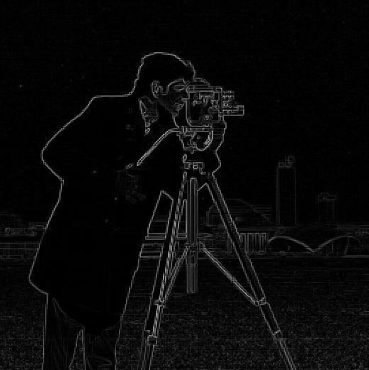
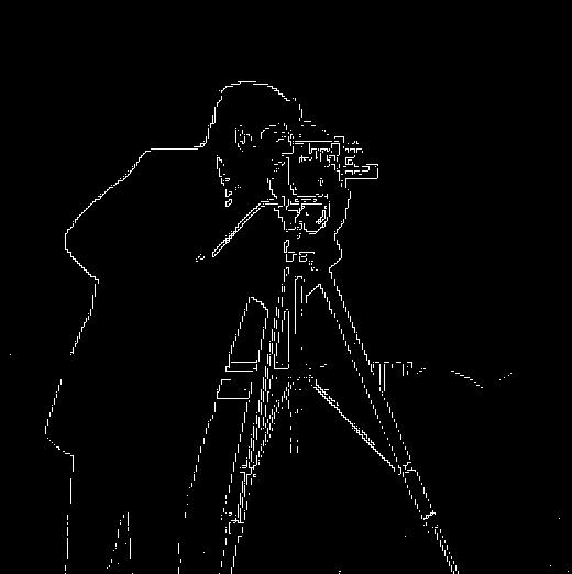
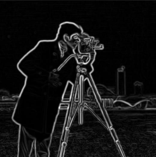
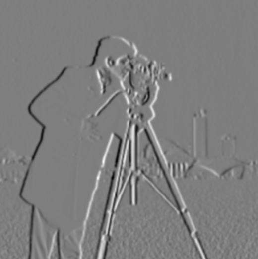
Fun with Filters and Frequencies!

"Know the white, but keep the black"

—Lao Tzu, Tao Te Ching (Feng/English trans.)

Part 1.1: Finite Difference Operator

A simple way to find edges in an image (such as, e.g., the cameraman image in Fig. 1a) is to threshold the magnitude of the gradient. We can calculate the (discrete) gradient magnitude by \(\|\nabla I\|=\sqrt{\left(\frac{\partial I}{\partial x}\right)^2+\left(\frac{\partial I}{\partial y}\right)^2}\), where \(\frac{\partial I}{\partial x}=D_x*I\) is the discrete \(x\)-gradient (Fig. 1b), computed by convolving the image with the horizontal finite difference kernel, and \(\frac{\partial I}{\partial y}=D_y*I\) is the discrete \(y\)-gradient (Fig. 1c), computed by convolving the image with the vertical finite difference kernel. Using the formula above, we can find the gradient magnitude of the cameraman image (Fig. 1d), and by thresholding the gradient magnitude at an appropriate value (we found that \(0.32\) worked well empirically), we can obtain a simple edge image (Fig. 1e).

Fig. 1a. cameraman.png.	Fig. 1b. \(D_x*I\).	Fig. 1c. \(D_y*I\).	Fig. 1d. \(\|\nabla I\|\).	Fig. 1e. \(\|\nabla I\|\ge 0.32\).

Part 1.2: Derivative of Gaussian (DoG) Filter

By smoothing the image (e.g., convolving with a Gaussian kernel \(G\)) before calculating the gradients (Fig. 2a) (here, we used \(\sigma=2\)), we can reduce the noise present in the gradients and edge image (Fig. 2b-e). We note that the resulting edges are thicker and smoother, and there are fewer instances of spurious (false positive) edges in the thresholded image.

Fig. 2a. \(G*I\).	Fig. 2b. \(D_x*(G*I)\).	Fig. 2c. \(D_y*(G*I)\).	Fig. 2d. \(\|\nabla (G*I)\|\).	Fig. 2e. \(\|\nabla (G*I)\|\ge 0.06\).

Alternatively, we can compute the finite differences of the Gaussian kernel (obtaining the DoG kernels) before convolving with the image (Fig. 3a). The final results are identical since convolution is an associative operation.

Fig. 3a. \(D_x*G, D_y*G\).	Fig. 3b. \((D_x*G)*I\).	Fig. 3c. \((D_y*G)*I\).	Fig. 3d. \(\|\nabla (G*I)\|\).	Fig. 3e. \(\|\nabla (G*I)\|\ge 0.06\).

Note: all computed images are \([0,1]\)-normalized before exporting, and \(10\) px are cropped from each side to remove edge artifacts present in the original input image.

"... Far, near, high, low, no two parts alike."

—Su Dongpo, Written on the Wall of West Forest Temple (Weston trans.)

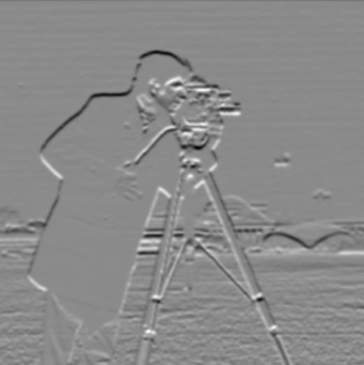
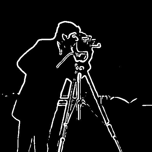
Part 2.1: Image "Sharpening"

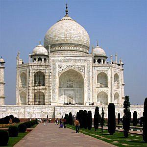
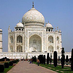
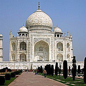
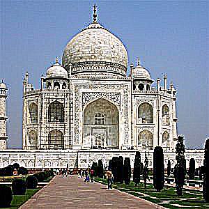
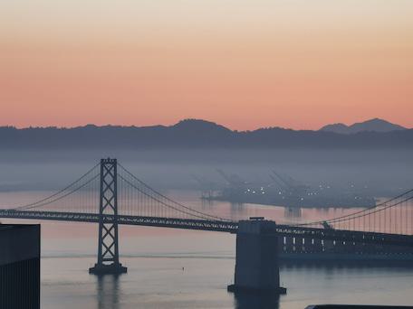
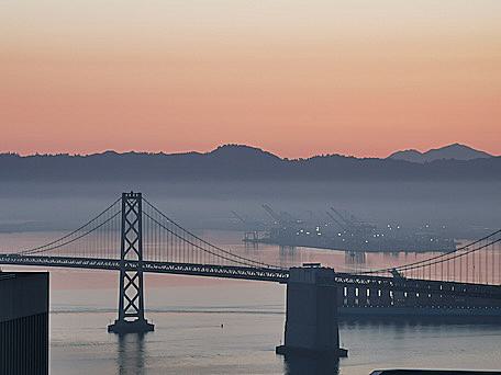
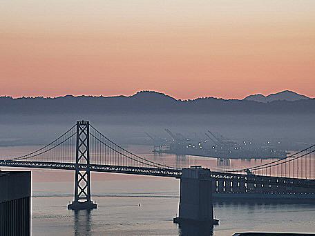
We can make an image appear sharper to the eye by adding more high frequency components. To do this, we derive the unsharp mask filter \(U_{\alpha,\sigma}:=\delta_{0,0}+\alpha(\delta_{0,0}-G_{0,0,\sigma})\), where \(\delta_{0,0}\) is the unit impulse filter and \(G_{0,0,\sigma}\) is a Gaussian filter. By convolving a given image with the unsharp mask filter, we can make it appear progressively sharper (Fig. 4a-b).

Legend	\(\alpha=0\) (Original)	\(\alpha=1\)	\(\alpha=2\)	\(\alpha=4\)	\(\alpha=8\)
Fig. 4a. taj.jpg.
Fig. 4b. bridge.

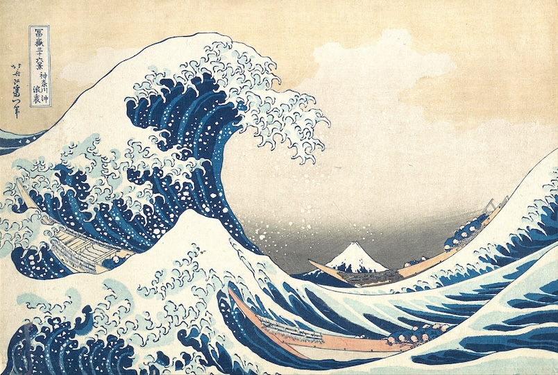
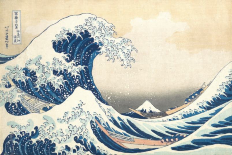
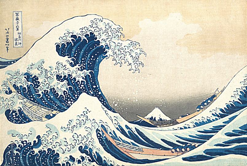
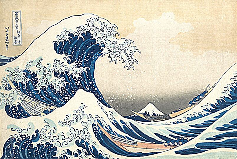
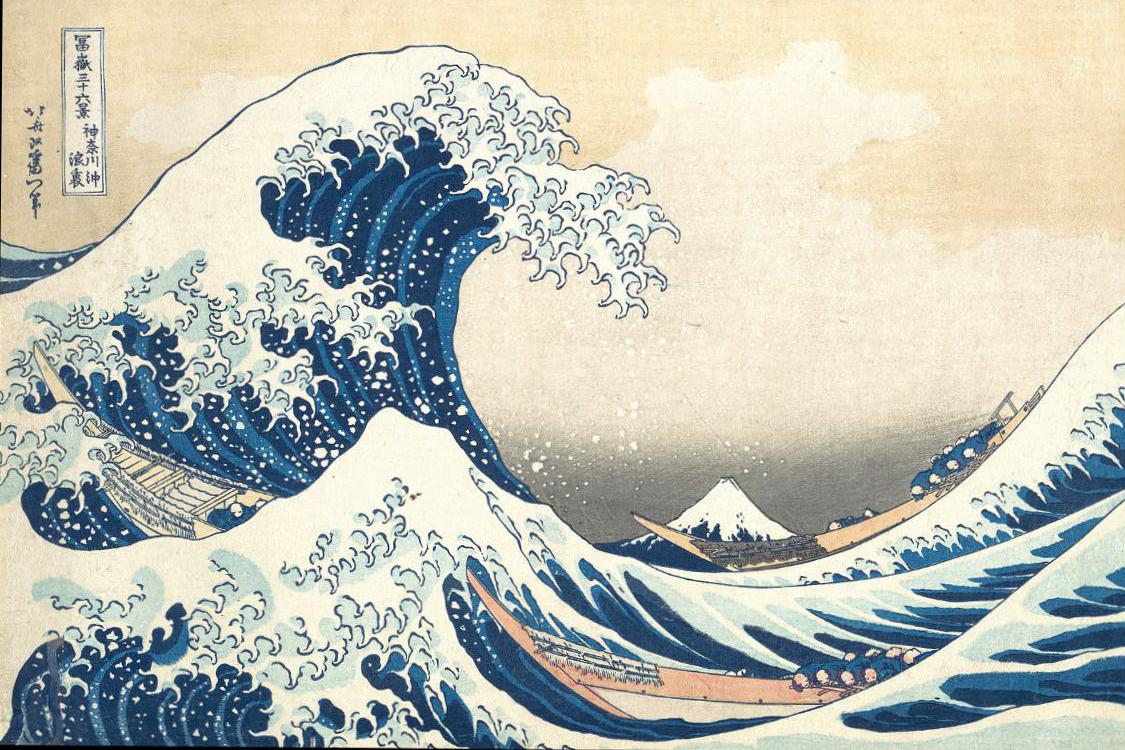
We also try to sharpen a blurred image (The Great Wave off Kanagawa, K. Hokusai, 1831, Woodblock print) using this method (Fig. 5). We note that the sharpening can introduce some artifacts (in the form of speckles or lines), that it makes edges more pronounced, and that it is unable to recover some of the information in the original image that was lost during the blurring process (such as the text).

Legend	Original	Blurred	\(\alpha=1\)	\(\alpha=2\)	\(\alpha=4\)	\(\alpha=8\)	Original
Fig. 5. wave.

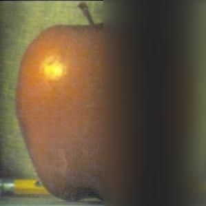
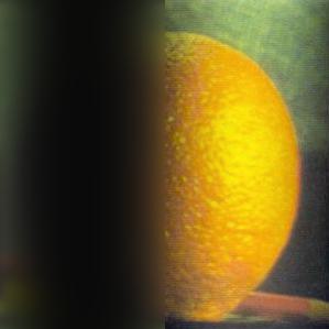
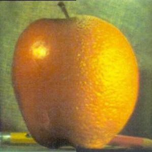
Part 2.2: Hybrid Images

We can create hybrid images by combining the low frequency components of one image with the high frequency components of anoter (cf. Oliva, Torralba, and Schyns, SIGGRAPH 2006). One efficient implementation takes the Fourier transform of both images \(\mathcal{F}(I_1), \mathcal{F}(I_2)\) and filters \(\mathcal{F}(G), \mathcal{F}(\delta_{0,0}-G)\), and takes a component-wise linear combination of the two images in the frequency domain \(\mathcal{F}(G)\mathcal{F}(I_1)+\mathcal{F}(\delta_{0,0}-G)\mathcal{F}(I_2)\). By the Fourier convolution theorem, this is equivalent to the Fourier transform of a superposition of the convolved images, which we can then translate back to the spatial domain by taking an inverse Fourier transform.
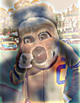
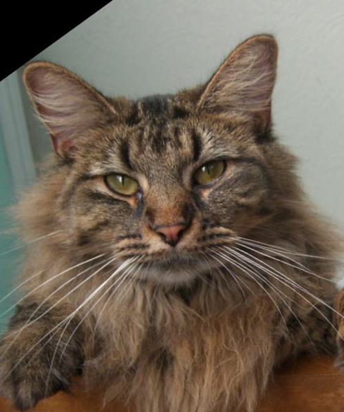
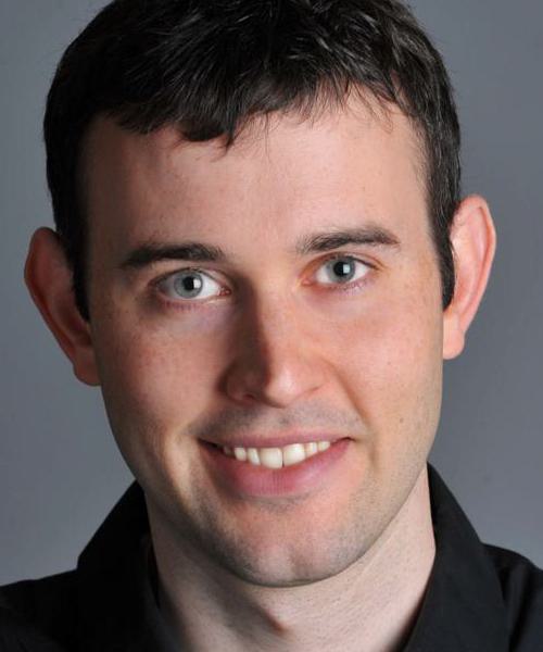
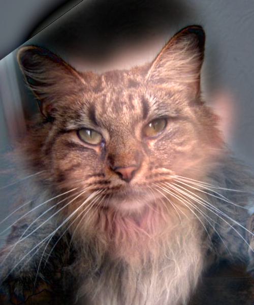
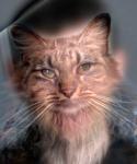
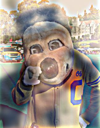
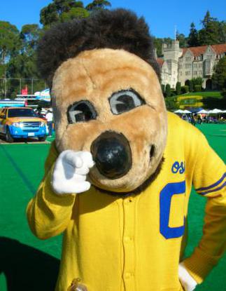
In our visualizations below, we show an image pyramid to simulate successively further viewing distances. Indeed, we find that the hybrid effect works well for the example of Derek and Nutmeg (Fig. 6a). We can create a similar effect by combining an image of Oski (Wikipedia) with the well-known Uncle Sam (J. M. Flagg, 1917, Lithograph) (Fig. 6b). We note that the effect works quite well, likely due to the similar expressions of the two characters.

Legend	Original	Hybrid
Fig. 6a. DerekPicture and nutmeg.
Fig. 6b. oski-wants-you.

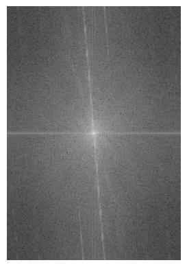
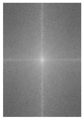
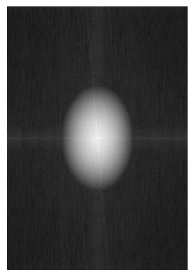
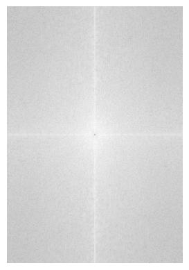
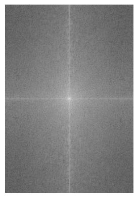
We visualized the process of creating a hybrid image (oski-wants-you) by showing the log magnitude of the Fourier transform of the two input images (Fig. 7a-b), the low-pass and high-pass filtered images (Fig. 7c-d), and the hybrid image (Fig. 7e).

Fig. 7a. \(\mathcal{F}(\text{uncle-sam})\).	Fig. 7b. \(\mathcal{F}(\text{oski})\).	Fig. 7c. \(\mathcal{F}(G*\text{uncle-sam})\).	Fig. 7d. \(\mathcal{F}((\delta_{0,0}-G)*\text{oski})\).	Fig. 7e. \(\mathcal{F}(G*\text{uncle-sam}+(\delta_{0,0}-G)*\text{oski})\).

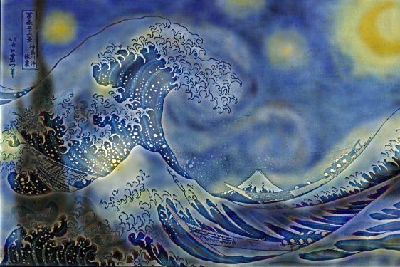
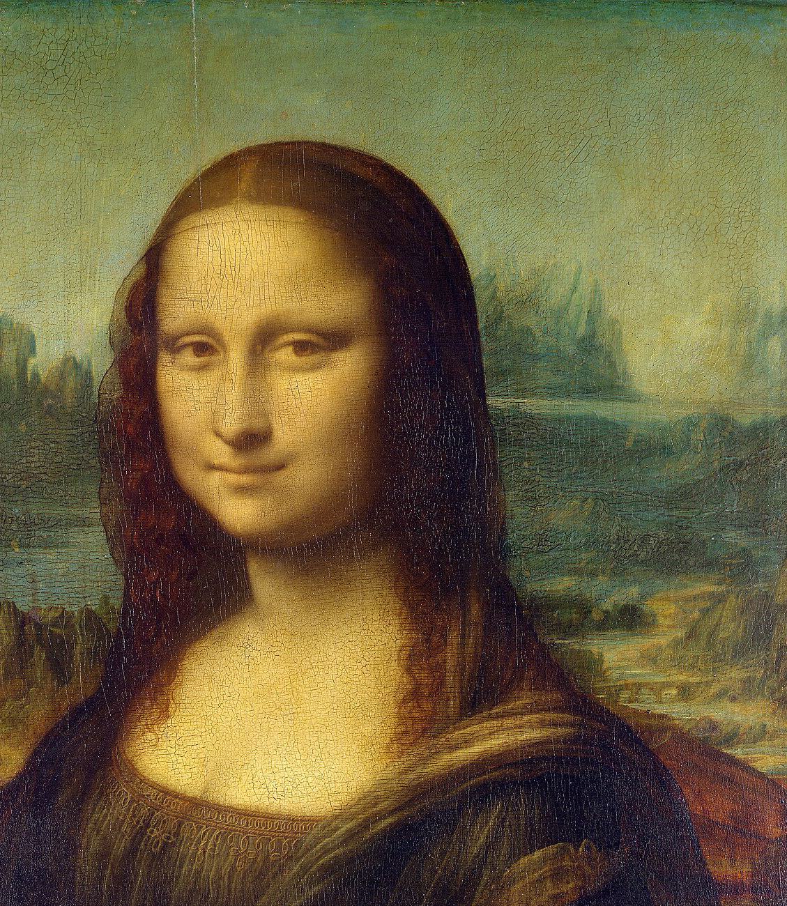
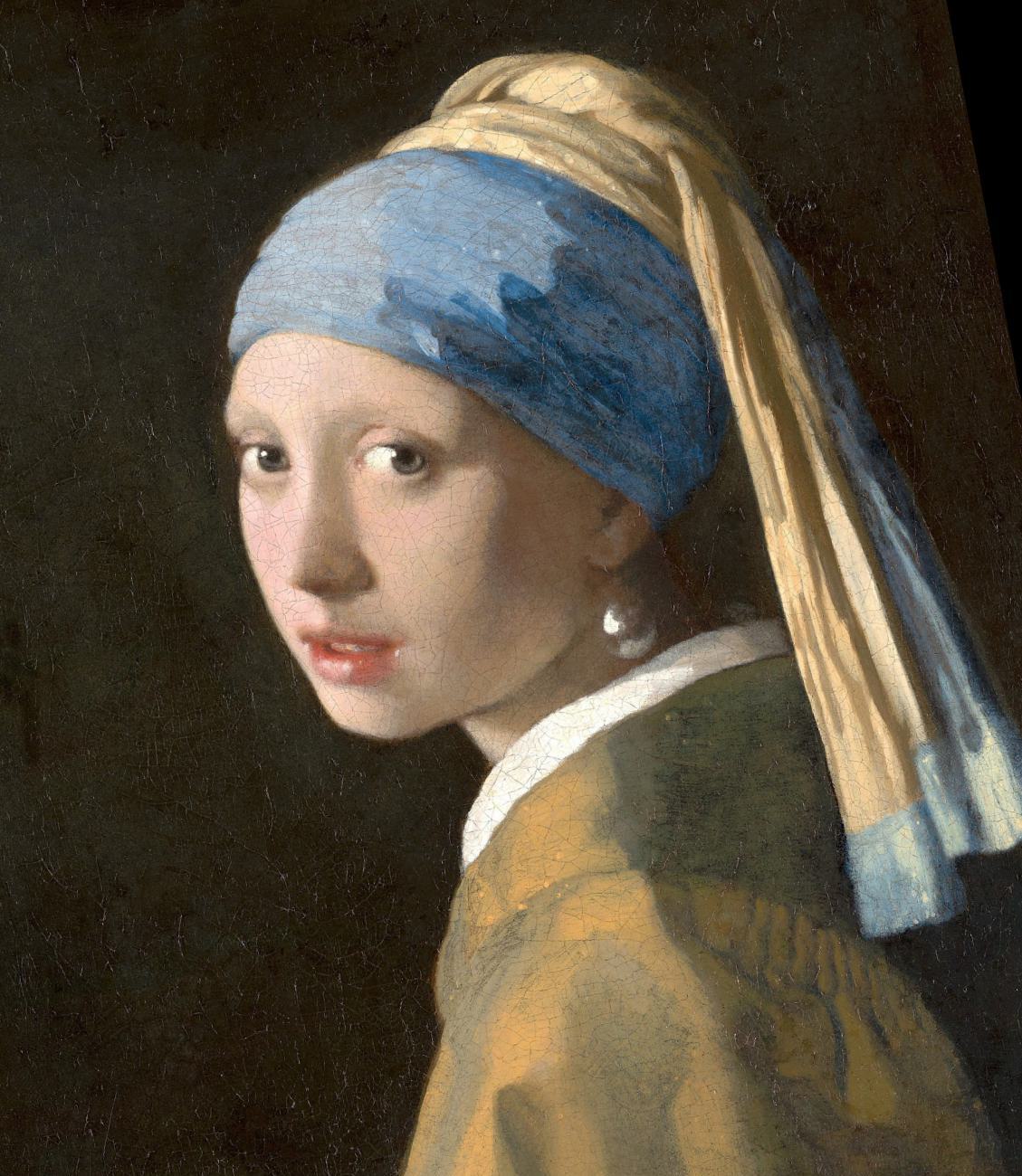
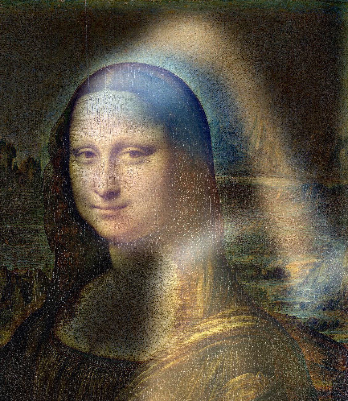
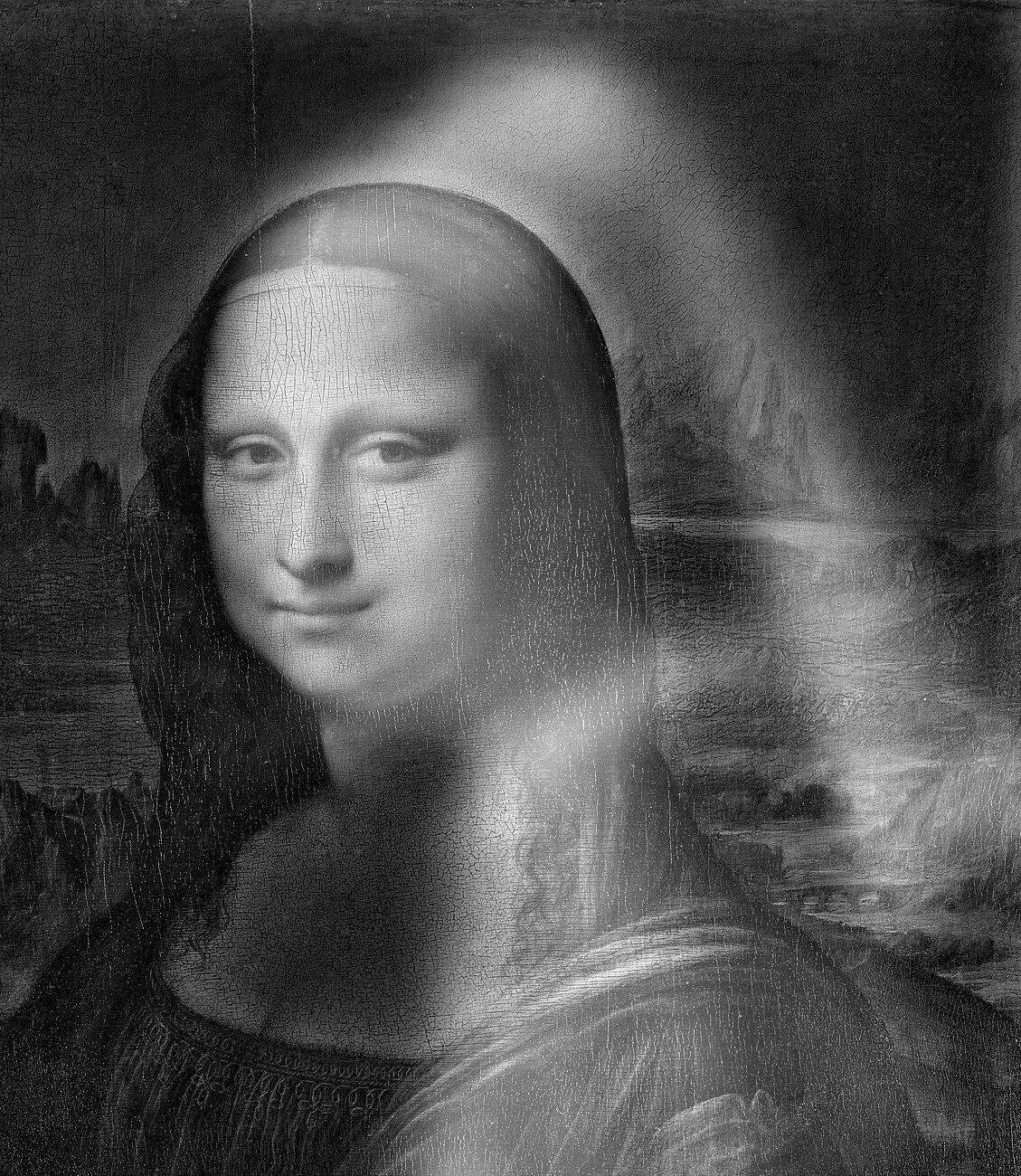
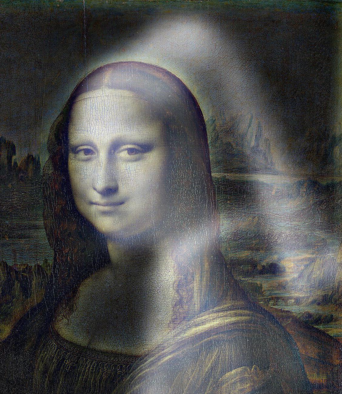
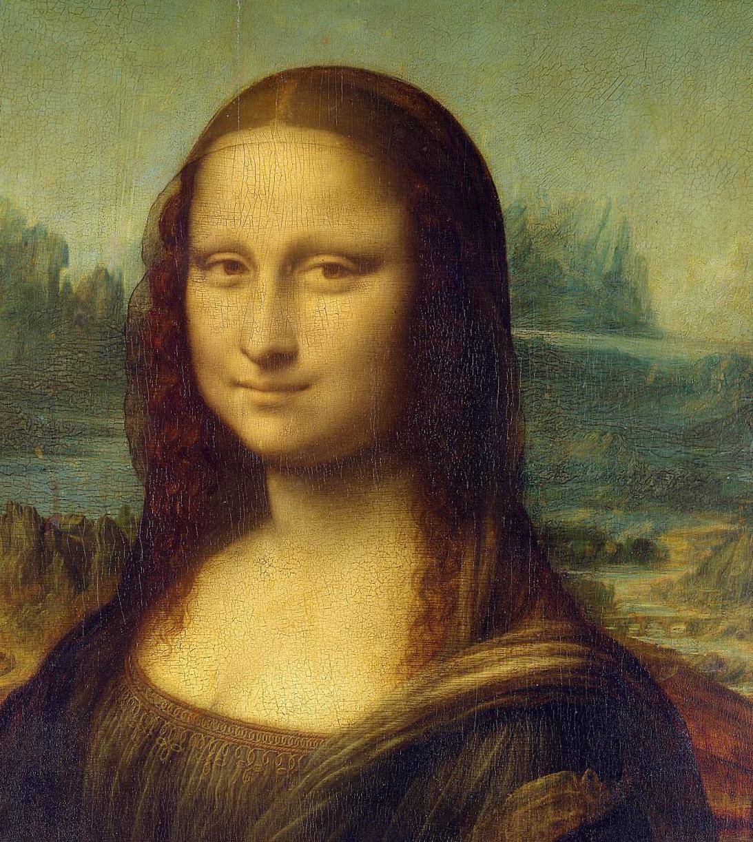
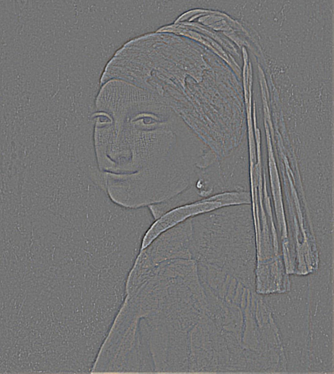
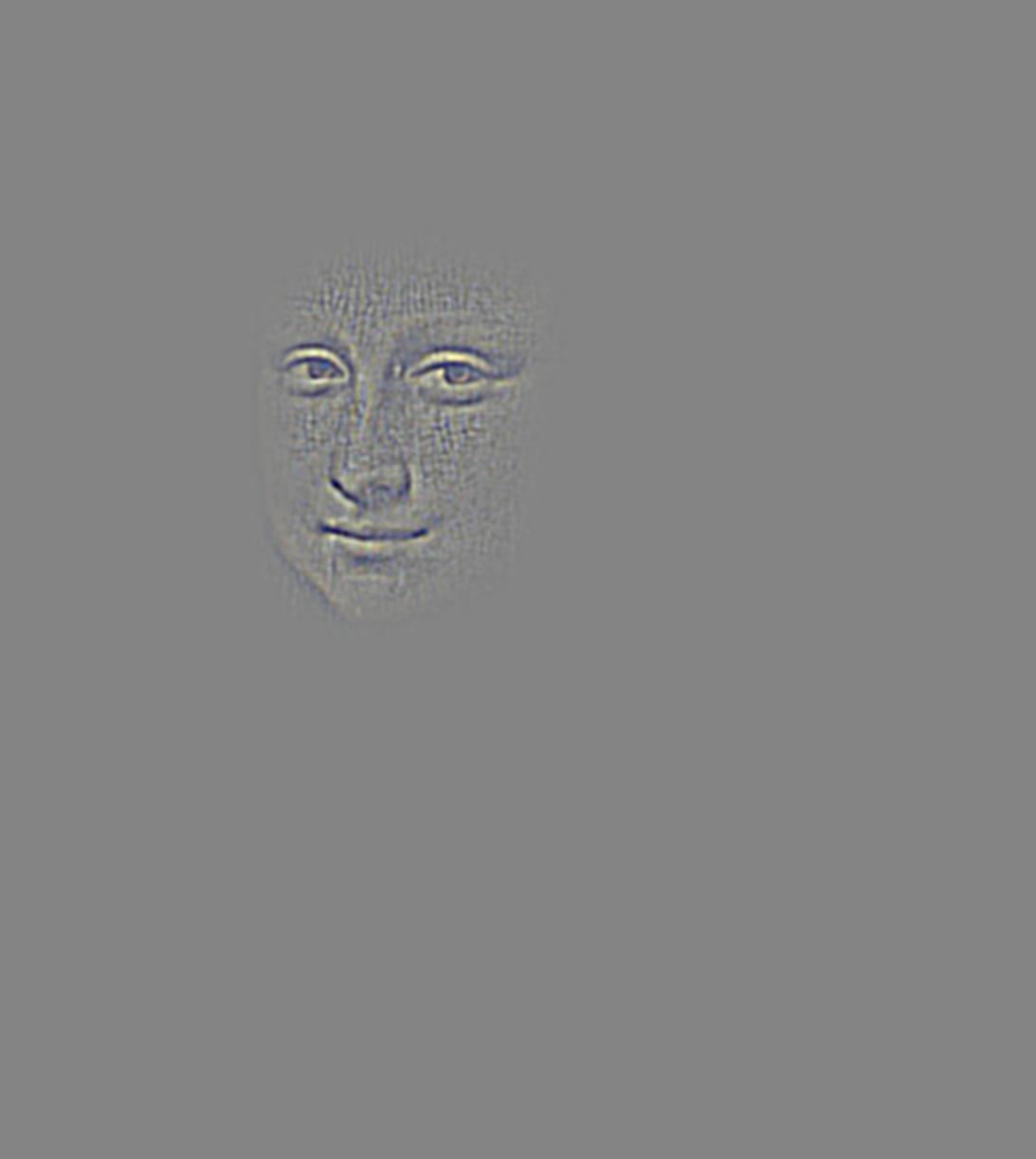
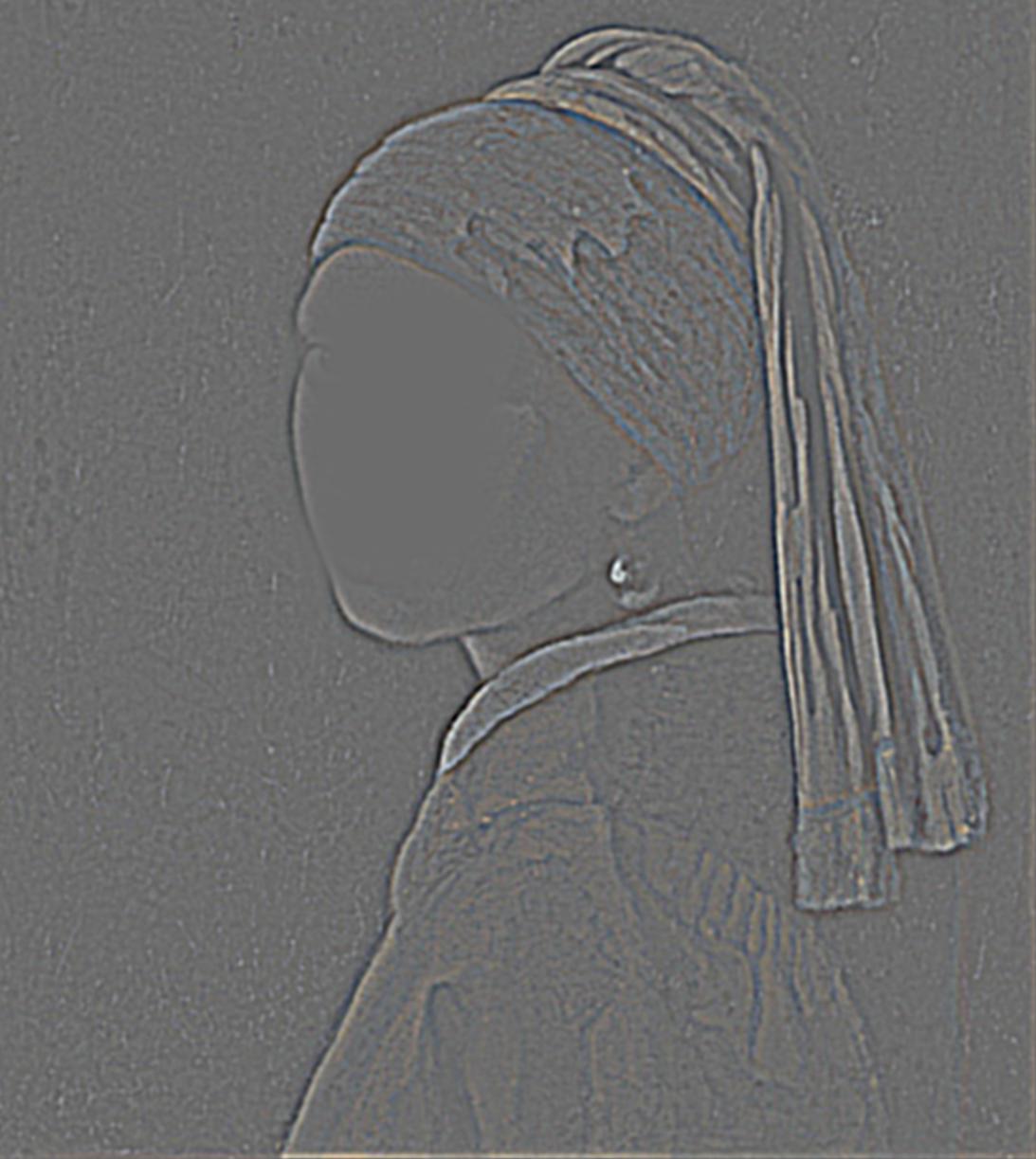
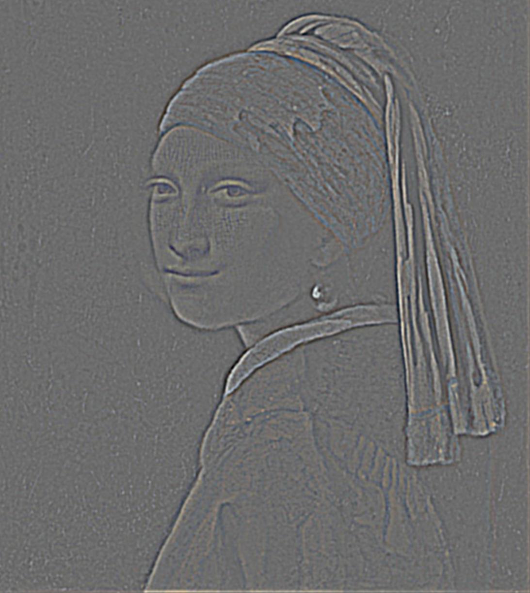
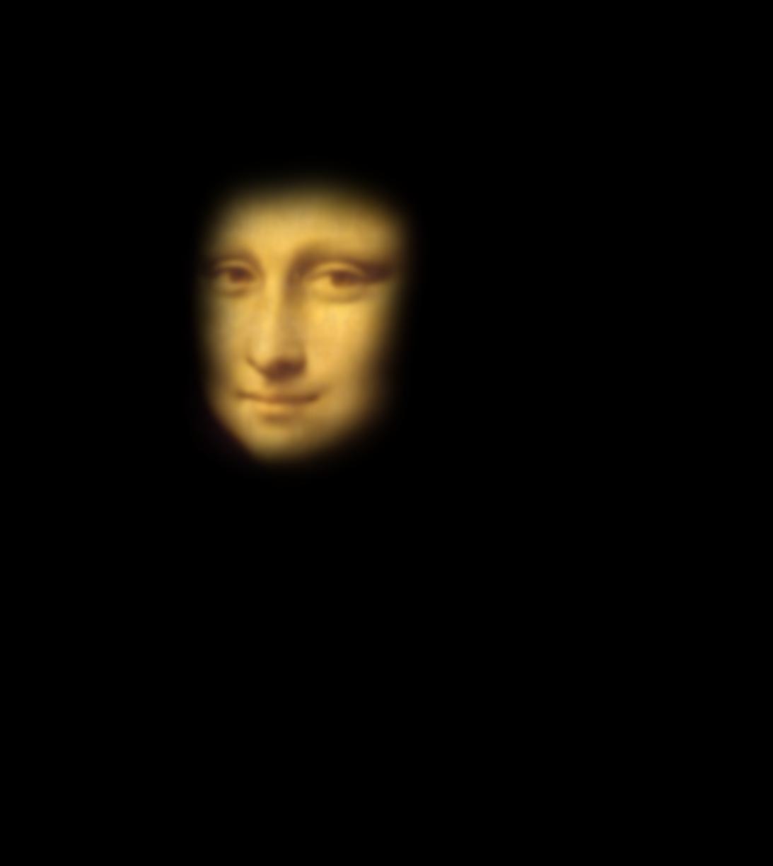
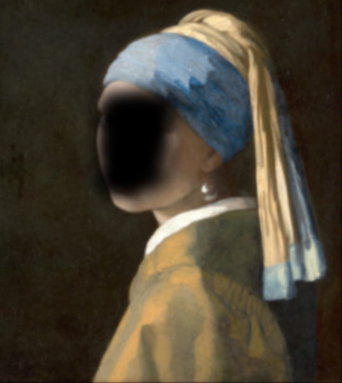
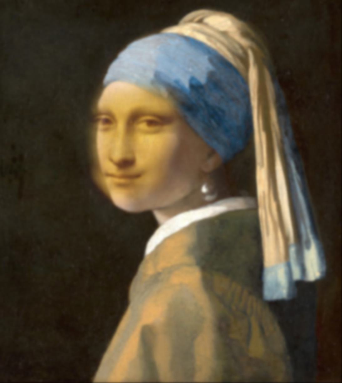
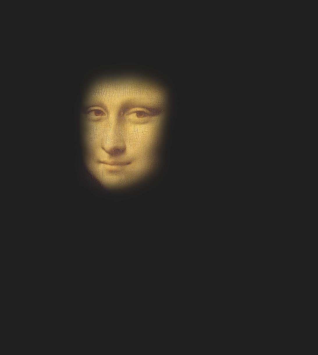
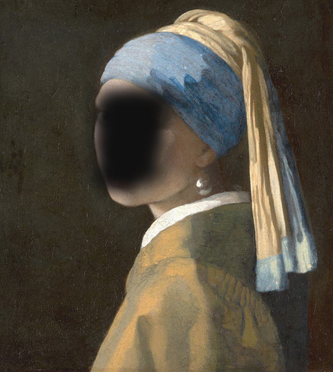
The effect also works for images that differ in style. We created a hybrid of The Great Wave off Kanagawa (K. Hokusai, 1831, Woodblock print) and Starry Night (V. van Gogh, 1889, Oil on canvas) (Fig. 8a), as well as a hybrid of the Mona Lisa (L. da Vinci, c. 1503-1506, Oil on poplar panel) and Girl with a Pearl Earring (J. Vermeer, c. 1665, Oil on canvas) (Fig. 8b).

Legend	Original	Hybrid
Fig. 8a. wavy-night.
Fig. 8a. mona-lisa-with-a-pearl-earring.

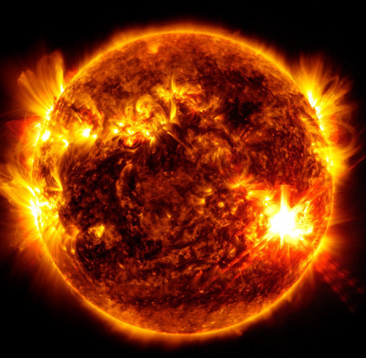
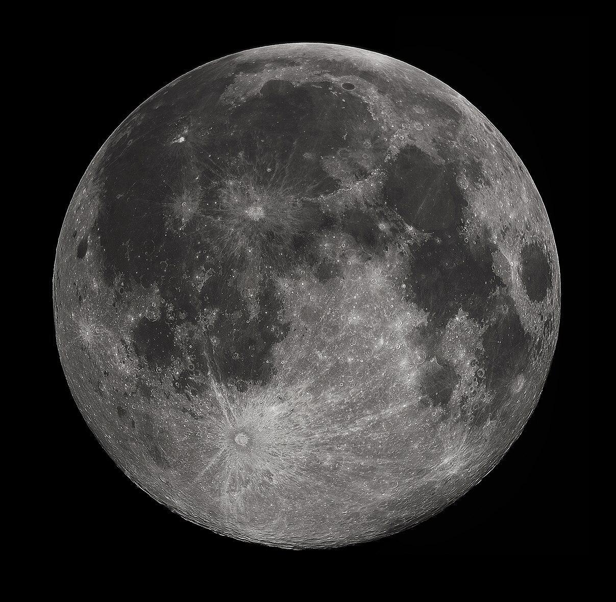
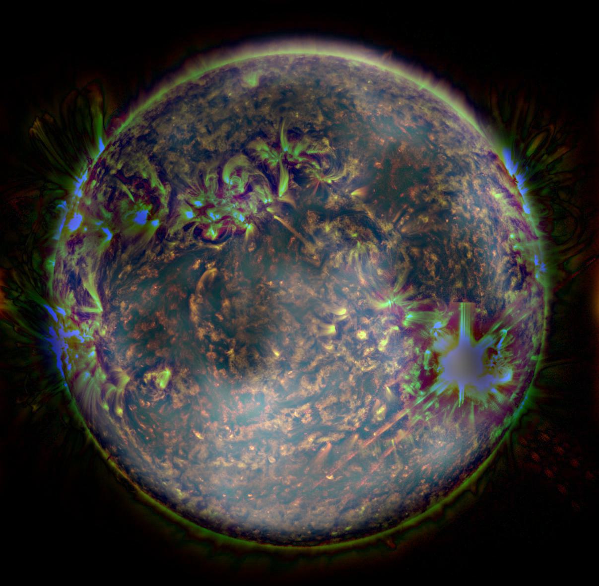
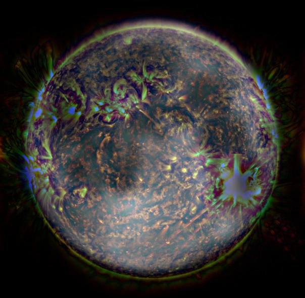
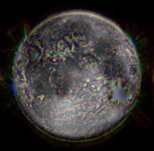
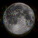
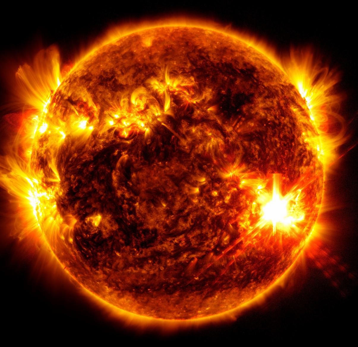
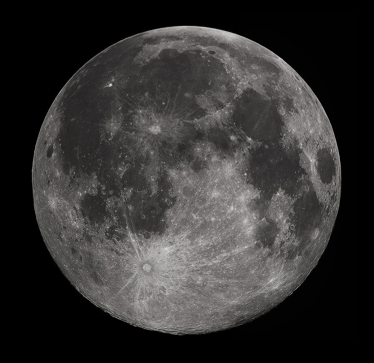
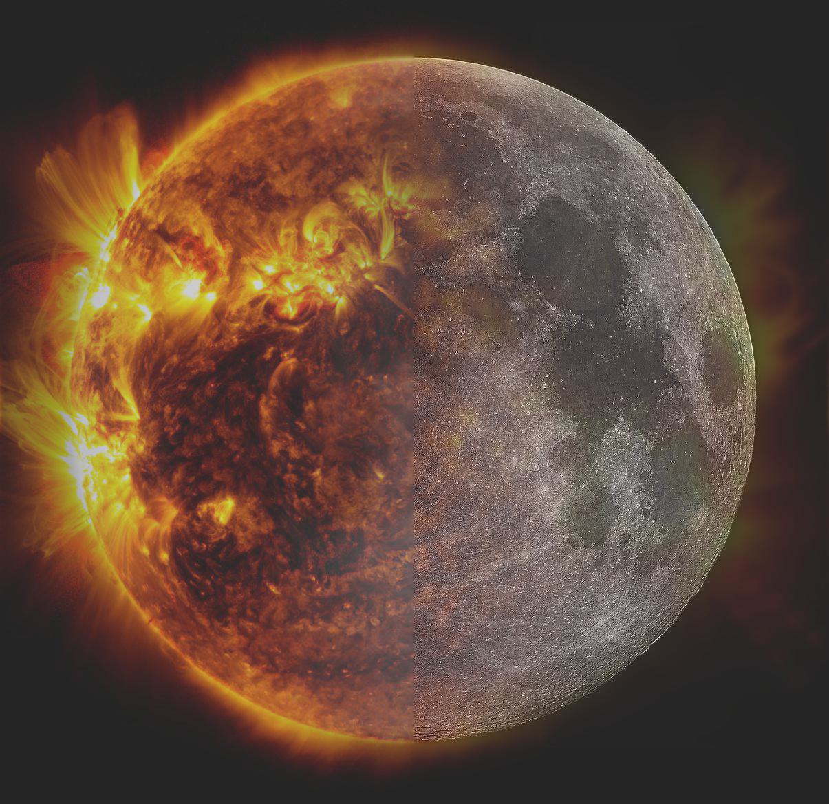
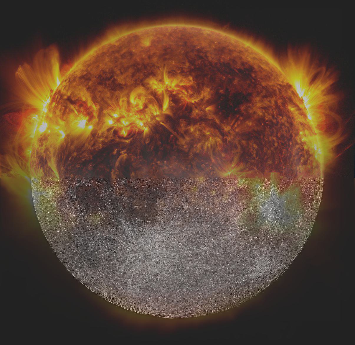
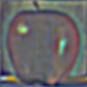
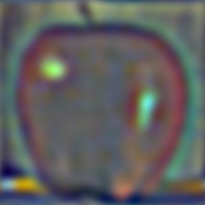
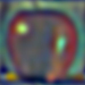
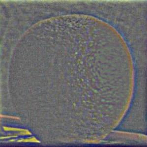
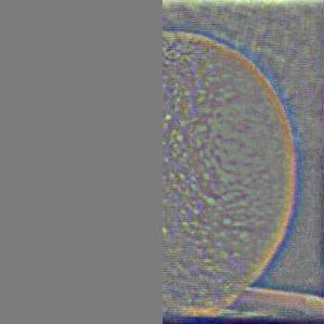
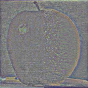
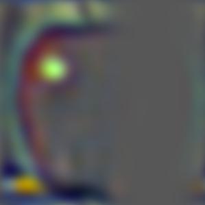
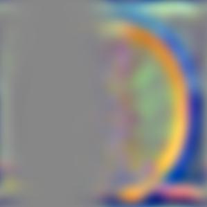
However, there are some limitations to the hybrid effect (failure cases). We were unable to produce a convincing hybrid image of the Sun and the Moon (Fig. 9). This is likely due to the two images both containing important information in high and low frequencies, and that they differ significantly in color (note that the sun appears to be tinted blue in the composite).

Legend	Original	Hybrid
Fig. 9. sunmoon.

Bells 🔔 and Whistles 🥳

We note that using color enhances the effect of the hybrid images (Fig. 10a-d). In particular, it seems best to include color for both images, especially when the images differ significantly in color scheme.

Fig. 10a. Both grayscale.	Fig. 10b. Low frequency color.	Fig. 10c. High frequency color.	Fig. 10d. Both color.

Part 2.3: Gaussian and Laplacian Stacks

We can create a Gaussian stack by successively applying a Gaussian filter to an input image (Fig. 11a-b). We can create a Laplacian stack by taking the difference of the Gaussian stack (Fig. 11c-d). This way, we can obtain a multi-frequency representation of the image (note that the original image is just the sum of the entire Laplacian stack and the last element of the Gaussian stack).

Legend	Stack Level 0	Stack Level 1	Stack Level 2	Stack Level 3	Stack Level 4	Stack Level 5	Stack Level 6	Stack Level 7	Stack Level 8	Stack Level 9
Fig. 11a. Gaussian stack of apple.jpeg.
Fig. 11b. Gaussian stack of orange.jpeg.
Fig. 11c. Laplacian stack of apple.jpeg.
Fig. 11d. Laplacian stack of orange.jpeg.

By applying a Gaussian stacked mask to each layer of the Laplacian stacks, we can recreate Fig. 3.42 in the Szelski textbook (which is adapted from Burt and Adelson, ACM TOG 1983) (Fig. 12):

	Fig. 12. Szelski Fig. 3.42.
(a)	(b)	(c)
(d)	(e)	(f)
(g)	(h)	(i)
(j)	(k)	(l)

Importantly, note that this multi-resolution blending scheme produces smooth transitions between the two images.

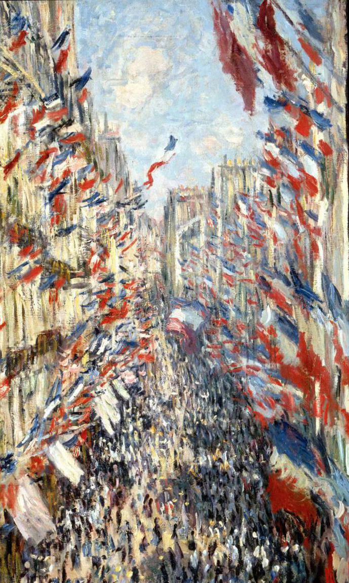
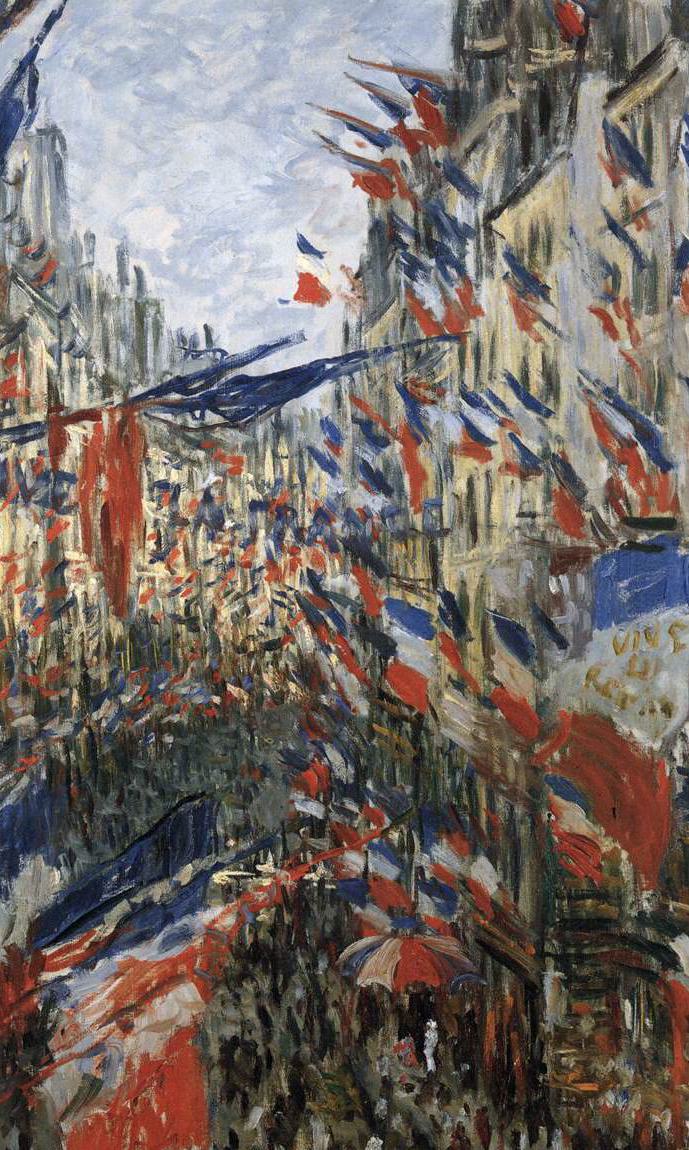
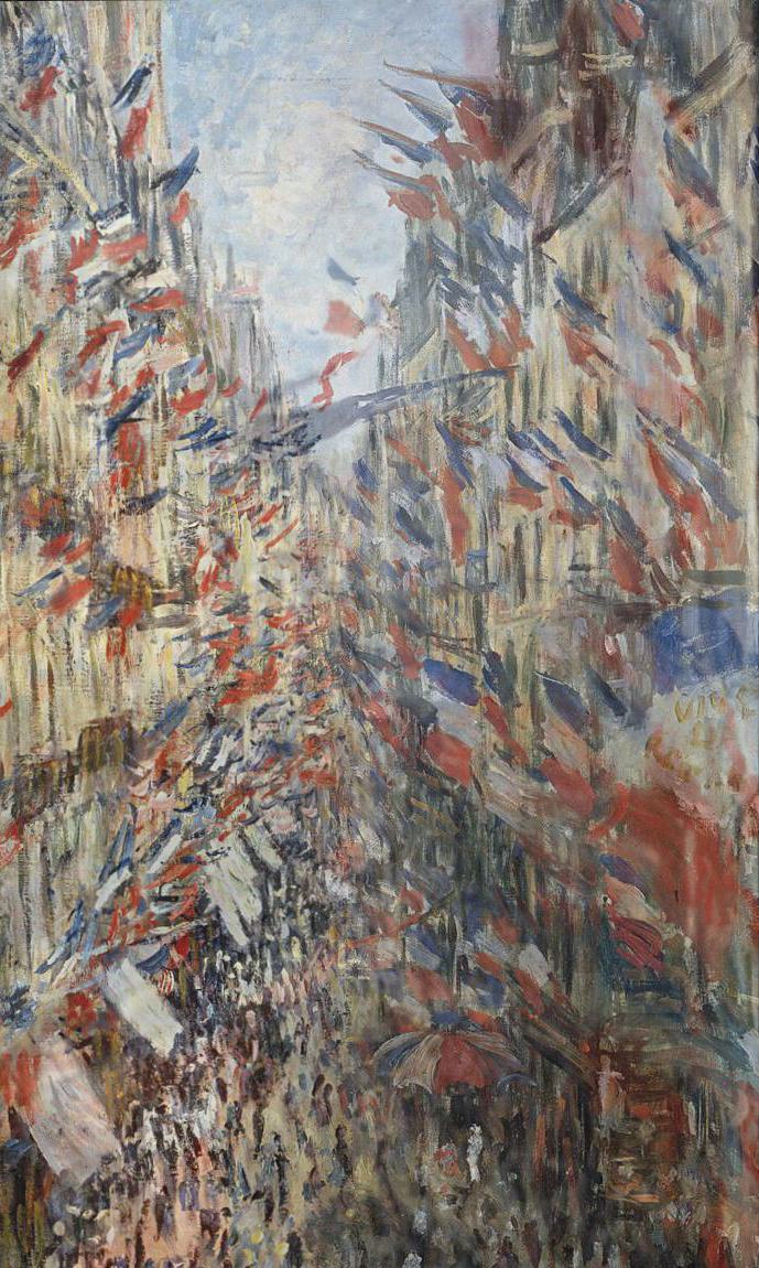
Part 2.4: Multiresolution Blending

Now, we can blend together arbitrary images by applying the multiresolution scheme above. For example, two streets in Paris: Rue Montorgueil (C. Monet, 1878, Oil on canvas), and Rue Saint-Denis (C. Monet, 1878, Oil on canvas) (Fig. 13a-b).

Fig. 13a. Original images.	Fig. 13b. rue-montordenis.

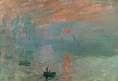
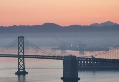
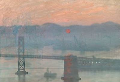
We also note that the blending scheme can be applied to images that differ in style, such as Impression, Sunrise (C. Monet, 1872, Oil on canvas), and a modern photo of sunrise over the Bay bridge (Fig. 14a-b).

Fig. 14a. Original images.	Fig. 14b. impressionist-bay-bridge.

We also reconsider the failed sunmoon example from our frequency hybrid; we are now able to stitch the two images together side by side (Fig. 15a-c).

Fig. 15a. Sun, Moon.	Fig. 15b. sunmoon_lr.	Fig. 15c. sunmoon_ud.

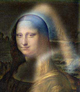
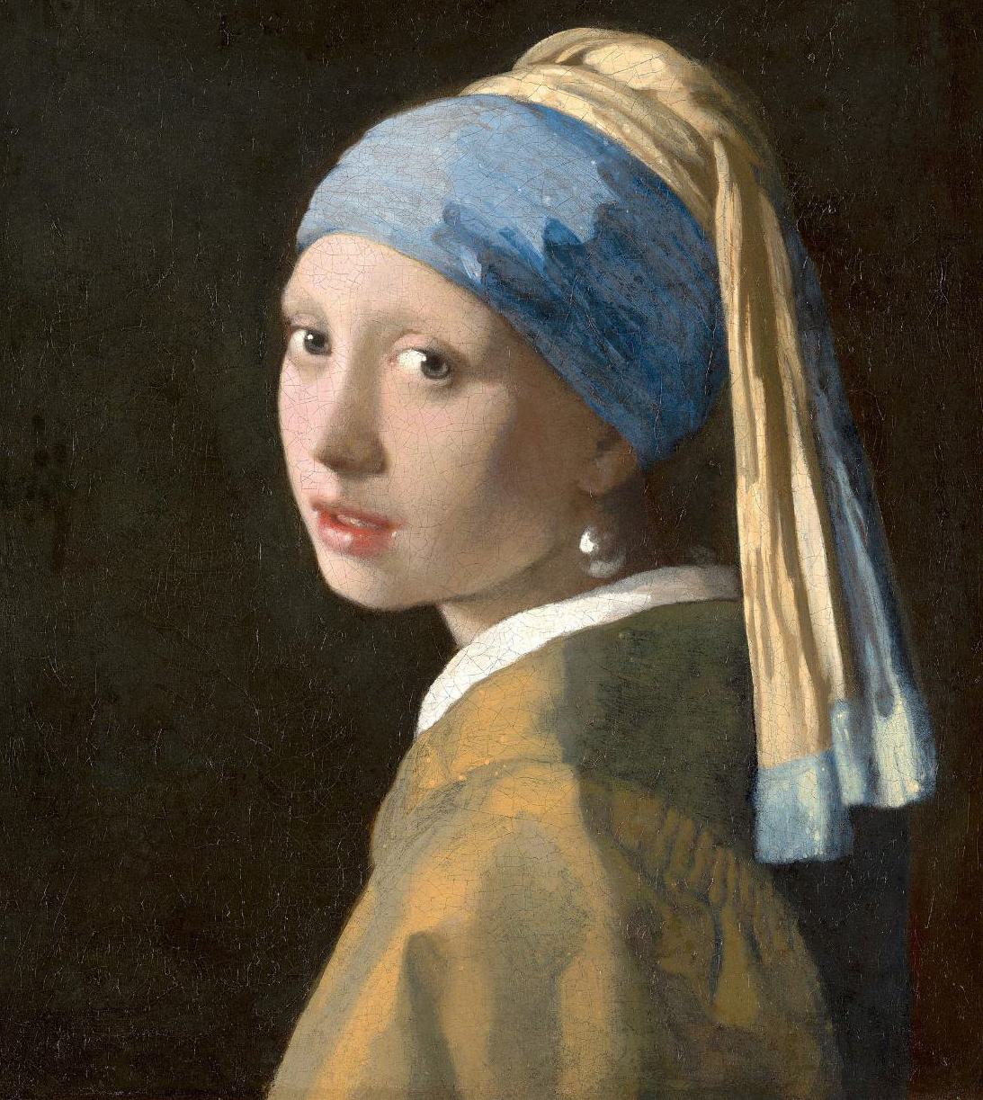
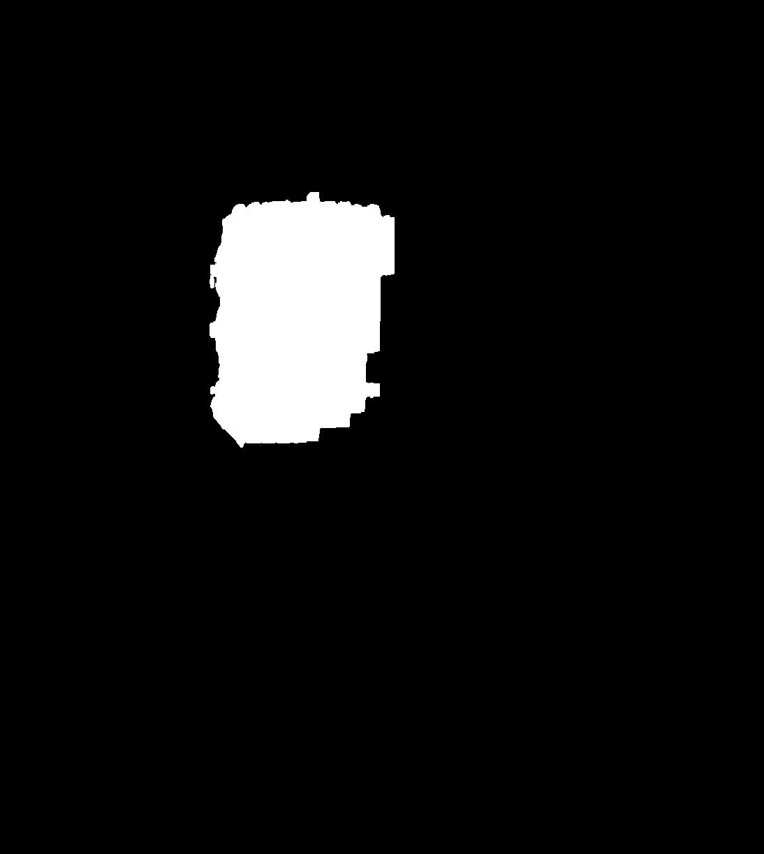
Finally, we revisit the mona-lisa-with-a-pearl-earring example, blending Mona Lisa (L. da Vinci, c. 1503-1506, Oil on poplar panel) and Girl with a Pearl Earring (J. Vermeer, c. 1665, Oil on canvas). With a custom mask extracted using SAM (note that we intentionally did not select the entire face but rather a ROI with non-smooth boundary), now information from both paintings can be perceived at the same viewing distance (Fig. 16a-c).

Fig. 16a. Original images.	Fig. 16b. Custom mask.	Fig. 16c. mona-lisa-with-a-pearl-earring.

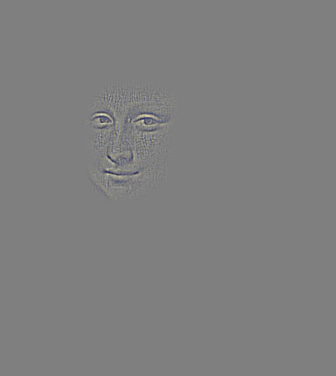
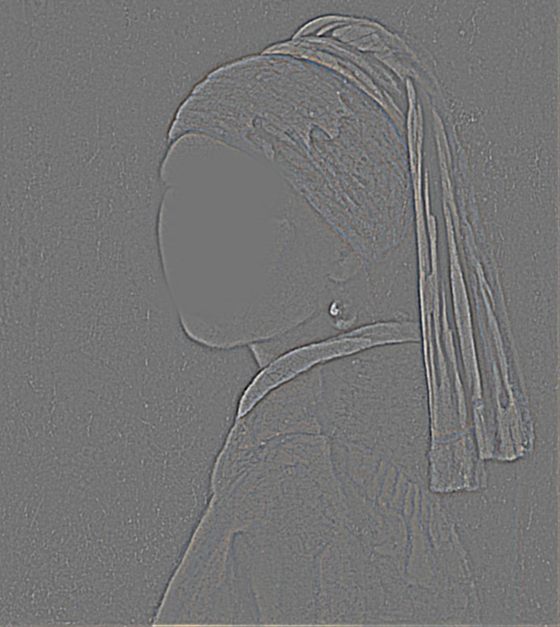
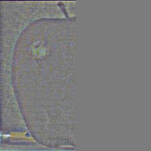
We demonstrate the multi-resolution blending process with a Szelski/Burt-Adelson type figure (Fig. 17). Note that we selected deeper levels in the stack for visualization since the superficial levels (high frequencies) were too faint due to the style of oil paintings.

	Fig. 17. Szelski Fig. 3.42.
(a)	(b)	(c)
(d)	(e)	(f)
(g)	(h)	(i)
(j)	(k)	(l)

Bells 🔔 and Whistles 🥳

Note that our implementation is able to process color images by default, and all of the preceding examples were done in color.

Comment: Exploiting human psychophysics

The reason underlying most of the effects produced in this project is that humans have different sensitivities for perceiving different spatial frequencies (cf. the Campbell-Robson curve). To a hypothetical observer with uniform sensitivity over the frequency domain, the hybrid images that we created would be equivalent to a linear combination of the two images (indeed, by the Fourier convolution theorem, the hybrid image is simply a superposition in frequency space). Therefore, ending our conclusion on a poetic note: why, as the Chinese poet Su Dongpo observed, does Mt. Lu appear "far, near, high, low, no two parts alike?" It is because human vision is not frequency invariant.