Fun with Diffusion Models!

"Leave the state that is well ordered and go to the state in chaos!"

—Chuang Tzu (Watson trans.)

Part 0: Setup

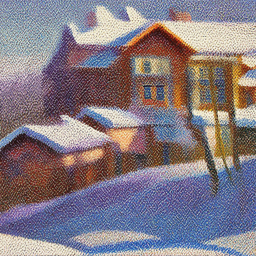
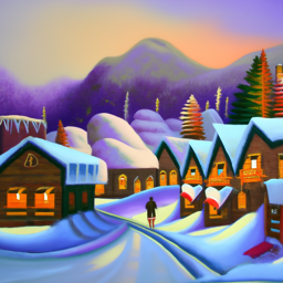
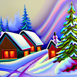
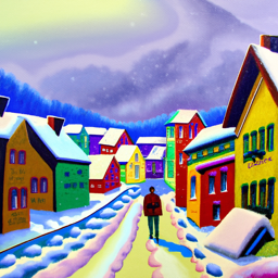
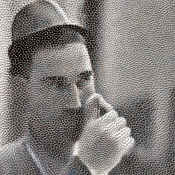
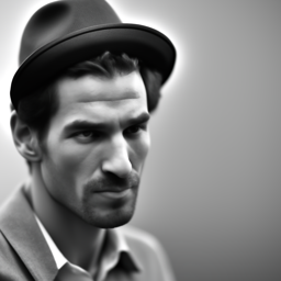
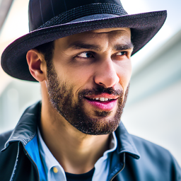
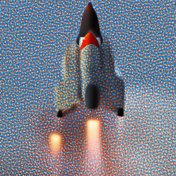
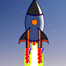
We obtain access to a pre-trained diffusion model (DeepFloyd IF). For this and all subsequent parts, we use random seed \(180\) for reproducibility. We sample from the model with three provided text prompts: an oil painting of a snowy mountain village, a man wearing a hat, and a rocket ship with various num_inference_steps values, and show the model outputs in Fig. 1. We note that the perceived image quality generally improves with larger num_inference_steps.

Prompt	\(5\) steps	\(10\) steps	\(20\) steps	\(40\) steps
an oil painting of a snowy mountain village
a man wearing a hat
a rocket ship

Part 1: Sampling Loops

In this part, we implement different variations of sampling procedures that use the pre-trained denoiser model to generate images under different conditions.

Part 1.1. Implementing the forward process

We implement the forward process of diffusion, which just adds noise to an image \(x_0\): \[x_t=\sqrt{\bar{\alpha_t}}x_0+\sqrt{1-\bar{\alpha_t}}\epsilon,\quad \epsilon\sim\mathcal{N}(0,1)\] Where \(\bar{\alpha_t}\) is determined by the noise schedule. We show the results from the forward process on a test image for \(t\in[250,500,750]\) (Fig. 2).

Original	\(t=250\)	\(t=500\)	\(t=750\)

Part 1.2. Classical denoising

We attempt to remove noise by filtering with a Gaussian. We show the best results that we were able to obtain (with \(\sigma=11\)) in Fig. 3 (each column shows noisy \(\rightarrow\) blurred), but note that it is difficult to recover the original image, especially when noise levels area high.

Original	\(t=250\)	\(t=500\)	\(t=750\)
	\(\rightarrow\)	\(\rightarrow\)	\(\rightarrow\)

Part 1.3. One-step denoising

We can also use the pre-trained denoiser model to estimate the noise present in the image and remove it appropriately. We show the results of this process in Fig. 4 (each column shows noisy \(\rightarrow\) one-step denoised).

Original	\(t=250\)	\(t=500\)	\(t=750\)
	\(\rightarrow\)	\(\rightarrow\)	\(\rightarrow\)

Part 1.4. Iterative denoising

We can iteratively denoise the image by applying the noise estimation and removal process multiple times, following the formula below and a given noise schedule. \[x_{t'}=\frac{\sqrt{\bar{\alpha_{t'}}\beta_{t}}}{1-\bar{\alpha_{t}}}x_0+\frac{\sqrt{\alpha_t}(1-\bar{\alpha_{t'}})}{1-\bar{\alpha_{t}}}x_t+v_{\sigma}\] We show results for iterative denoising, as well as comparisons to the methods in previous parts, in Fig. 5. Indeed, iterative denoising produces a less blurry image than one-step denoising.

\(t=690\)	\(t=540\)	\(t=390\)	\(t=240\)	\(t=90\)	Iterative denoised (\(t=0\))	Original	One-step denoised	Gaussian blurred

Part 1.5. Diffusion model sampling

We can generate images by running the iterative denoising procedure starting from pure noise (the largest time point). Some results are shown below in Fig. 6.

Sampled images

Part 1.6. Classifier-free guidance

We can improve the quality of our generated images by implementing classifier-free guidance, where we compute two noise estimates (one conditional and one unconditional) and use the linear combination \[\epsilon=\epsilon_u+\gamma(\epsilon_c-\epsilon_u)\] Where \(\gamma\) is a scalar parameter. We show the results of this process in Fig. 7 for \(\gamma=7\).

Sampled images

Part 1.7. Image-to-image translation

We can edit images by adding noise to them and then denoising them. We show the results of this process in Fig. 8 with different amounts of noise added (the index \(i\) that we use corresponds to that in strided_timesteps=range(990,-1,-30)).

Legend	i=1	i=3	i=5	i=7	i=10	i=20	Original
campanile
taj
gugong

Part 1.7.1. Editing hand-drawn and web images

Similarly, we can perform the above procedure on non-realistic images. Examples are shown in Fig. 9.

Legend	i=1	i=3	i=5	i=7	i=10	i=20	Original
camera
taj
gugong

Part 1.7.2. Inpainting

We can also use CFG to inpaint images, by forcing the image to be unambiguous outside the edit mask region: \[x_t\leftarrow mx_t + (1-m)]\text{forward}(x_{\text{orig}},t)\] We show the results of this process in Fig. 10.

Legend	Original	Mask	Inpainted
campanile
taj
bridge

Part 1.7.3. Text-conditional image-to-image translation

We can condition on a text prompt during SDEdit to generate hybrid images between the prompt and the original image. We show the results of this process in Fig. 11, where the text prompt is a rocket ship.

Legend	i=1	i=3	i=5	i=7	i=10	i=20	Original
campanile
taj
gugong

Part 1.8. Visual anagrams

We can generate visual anagrams by averaging noise estimates from different text prompts appropriately. We show the results of this process in Fig. 12.

Upright	Flip
an oil painting of people around a campfire	an oil painting of an old man
a man wearing a hat	a photo of a dog
an oil painting of a snowy mountain village	a photo of the amalfi cost

Part 1.9. Hybrid images

We can generate hybrid images by filtering noise estimates from different text prompts and taking the sum. We show the results of this process in Fig. 13.

Hybrid	Low Pass	High Pass
	a lithograph of a skull	a lithograph of waterfalls
	a lithograph of a skull	a photo of a dog
	a photo of a dog	an oil painting of people around a campfire

"... The ten thousand things would develop naturally.
If they still desired to act,
They would return to the simplicity of formless substance."

—Lao Tzu, Tao Te Ching (Feng/English trans.)

Part 1: Training a Single-Step Denoising UNet

We implement a UNet architecture for one-step denoising, where the loss is \[\mathcal{L}=\mathbb{E}_{z,x}\|D_{\theta}(z)-x\|_2^2.\] This can be trained with self-supervised learning, where we generate a noisy image \(z\) by adding Gaussian noise to the original image \(x\): \[z=x+\sigma\epsilon,\quad \epsilon\sim\mathcal{N}(0,I).\] We visualize the noising process in Fig. 14.

\(\sigma=0\)	\(\sigma=0.2\)	\(\sigma=0.4\)	\(\sigma=0.5\)	\(\sigma=0.6\)	\(\sigma=0.8\)	\(\sigma=1.0\)

We train the model on MNIST for \(5\) epochs with \(\sigma=0.5\), batch size \(256\), hidden dimension \(128\), and the Adam optimizer with learning rate \(10^{-4}\). We see that the loss decreases and the model converges (Fig. 15).

We show the results of the model after the first and fifth epoch in Fig. 16.

Original	Noisy (\(\sigma=0.5\))	Output (one epoch)	Output (five epochs)

We can also test the denoiser with varying levels of noise, and we show the results in Fig. 17.

Legend	\(\sigma=0\)	\(\sigma=0.2\)	\(\sigma=0.4\)	\(\sigma=0.5\)	\(\sigma=0.6\)	\(\sigma=0.8\)	\(\sigma=1.0\)
Noisy
Output

Part 2: Training a Diffusion Model

In this part, we implement DDPM with iterative denoising, where our UNet predicts the noise present in the image at a given timestep \(t\). We add time conditioning to our UNet by embedding the timestep \(t\) with Linear layers and adding it to the outputs of appropriate layers in the original UNet. During training, we pick a random \(t\) for each batch and predict the noise present in the image at that timestep. We train the model on MNIST for \(20\) epochs with batch size \(128\), hidden dimension \(64\), and the Adam optimizer with learning rate \(10^{-3}\) and exponential learning rate decay with \(\gamma=0.1^{1/20}\). We see that the loss decreases and the model converges (Fig. 18).

We can sample from the model by iteratively denoising pure noise, and we show the results of the model after the \(\{1,5,10,15,20\}\)th epochs in Fig. 19.

Epoch \(1\)	Epoch \(5\)	Epoch \(10\)	Epoch \(15\)	Epoch \(20\)

We also add class conditioning to the model by embedding the one-hot encoded class label \(c\) with Linear layers and multiplying it with the outputs of appropriate layers in the original UNet. To preserve the ability to generate unconditionally, we implement dropout of the class conditioning vector with probability \(p=0.1\). We again train the model on MNIST for \(20\) epochs with batch size \(128\), hidden dimension \(64\), and the Adam optimizer with learning rate \(10^{-3}\) and exponential learning rate decay with \(\gamma=0.1^{1/20}\). We see that the loss decreases and the model converges (Fig. 20).


We can now sample from the model conditioned on the digit class. We use CFG with \(\gamma=5\), and we show the results of the model after the \(\{1,5,10,15,20\}\)th epochs in Fig. 20.

Epoch \(1\)	Epoch \(5\)	Epoch \(10\)	Epoch \(15\)	Epoch \(20\)