(Auto)Stitching Photo Mosaics

Project 4A: Image Warping and Mosaicing

Part 1: Shoot and digitize pictures

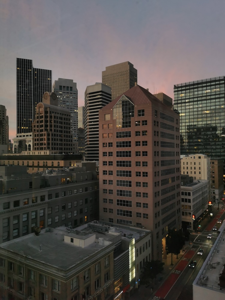
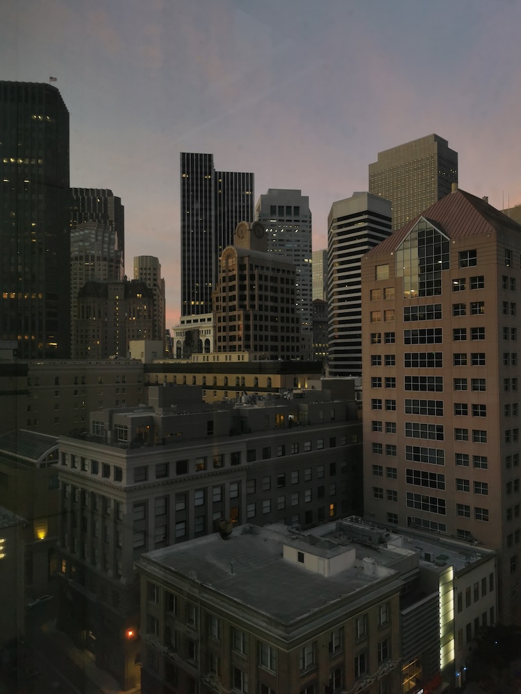
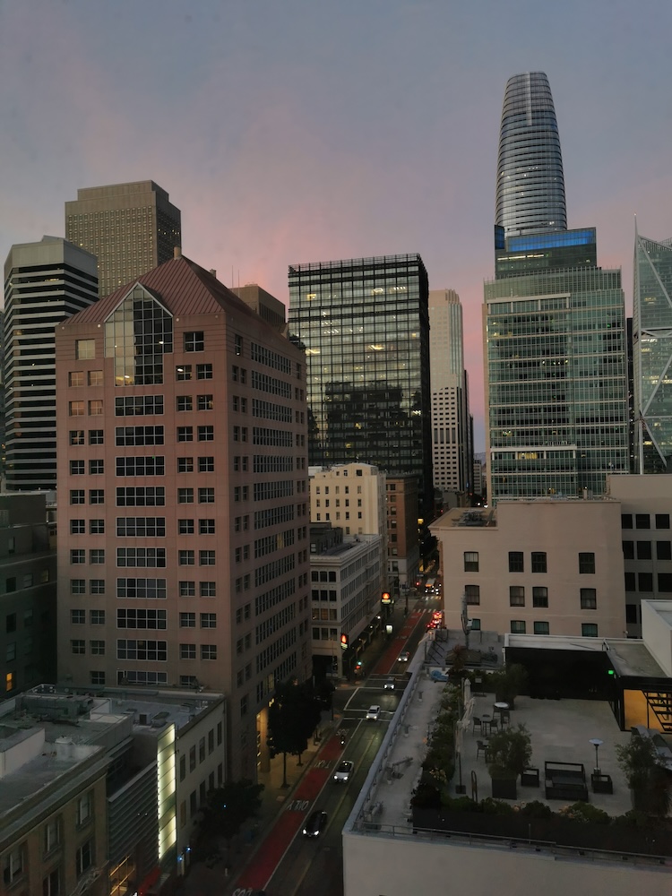
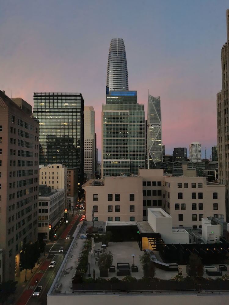
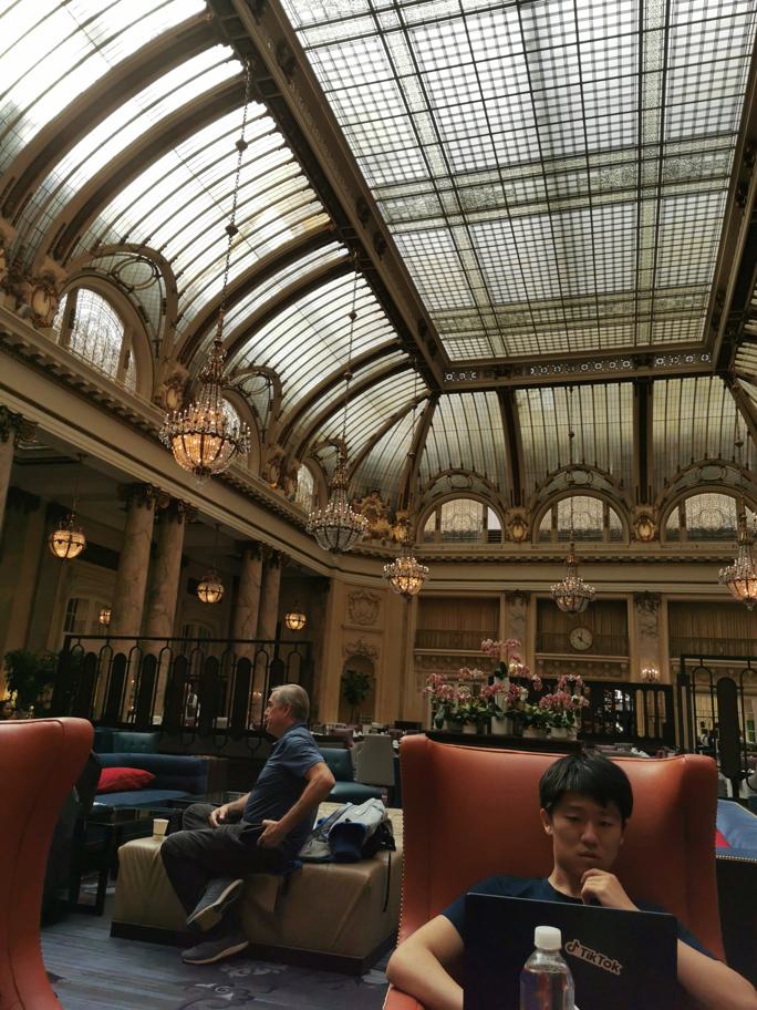
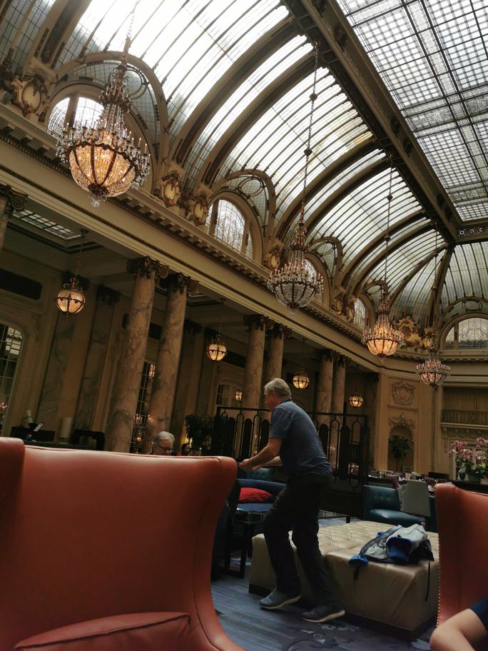
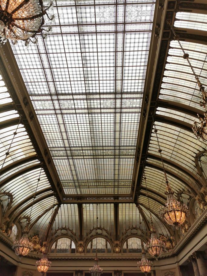
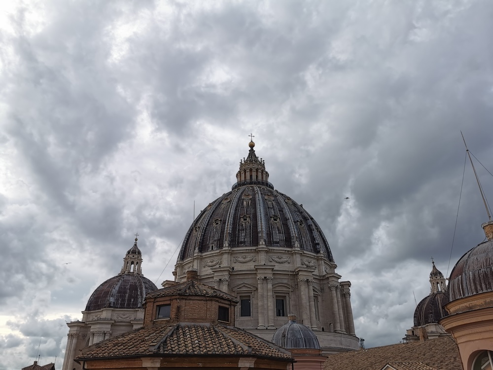
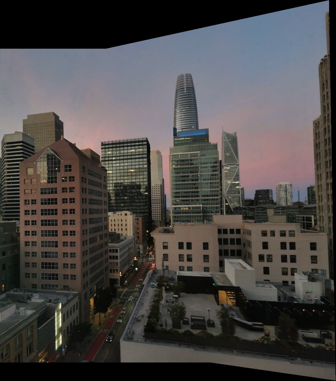
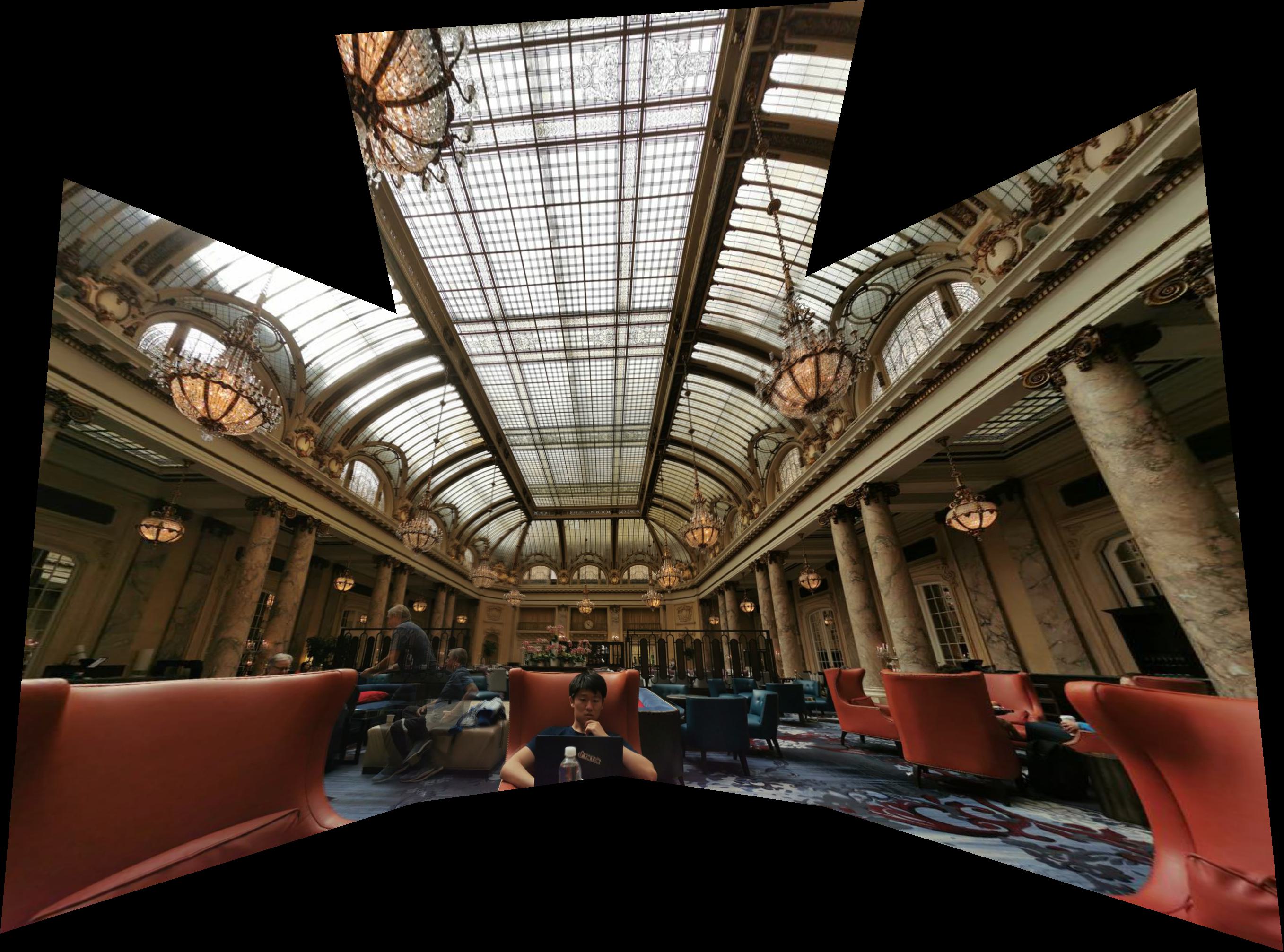
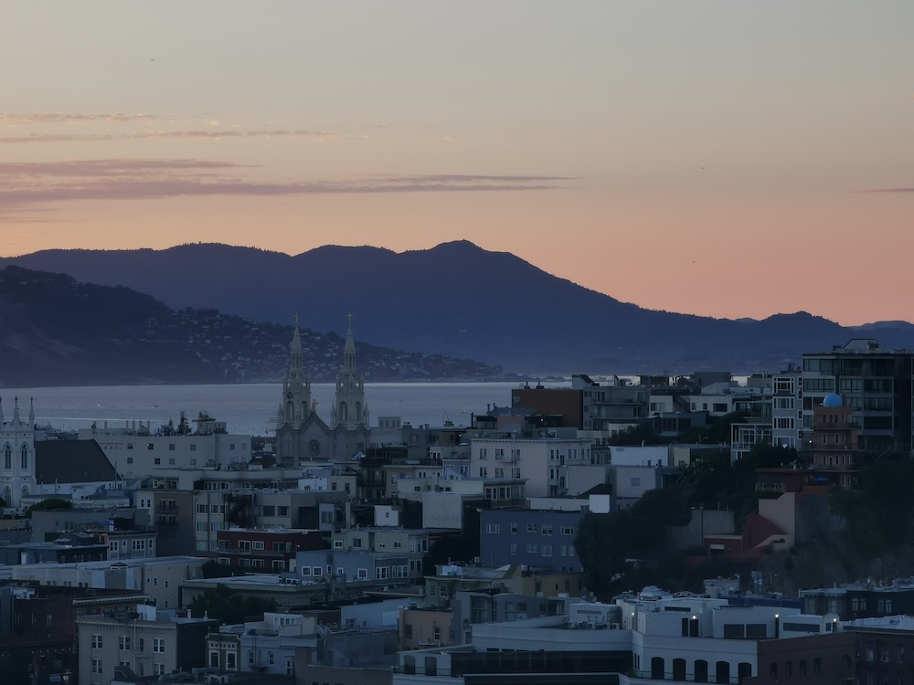
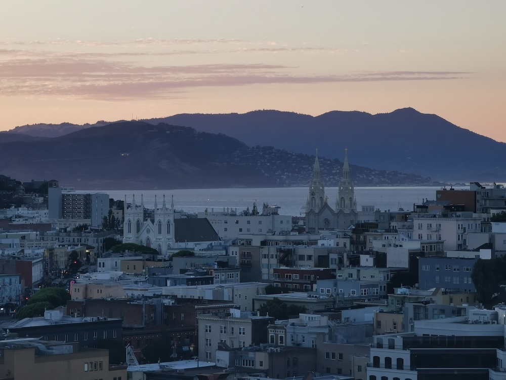
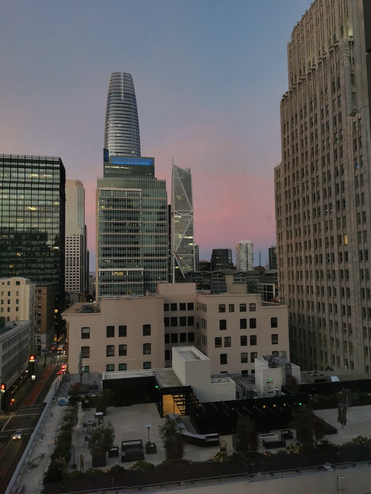
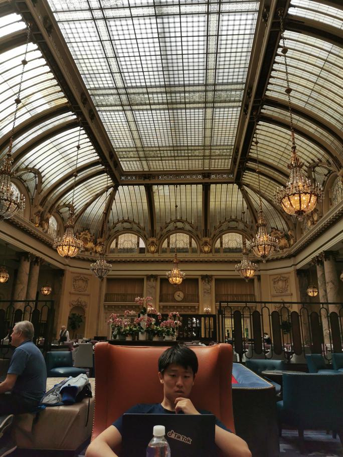
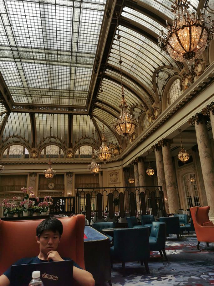
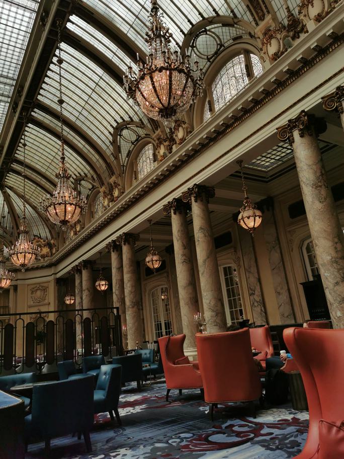
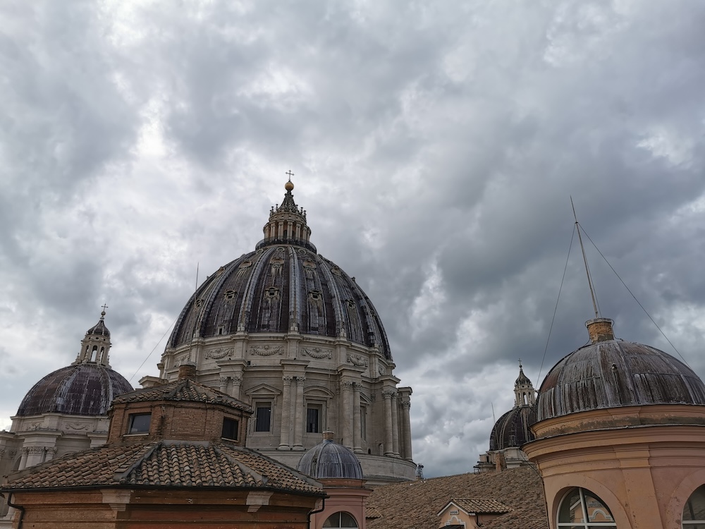
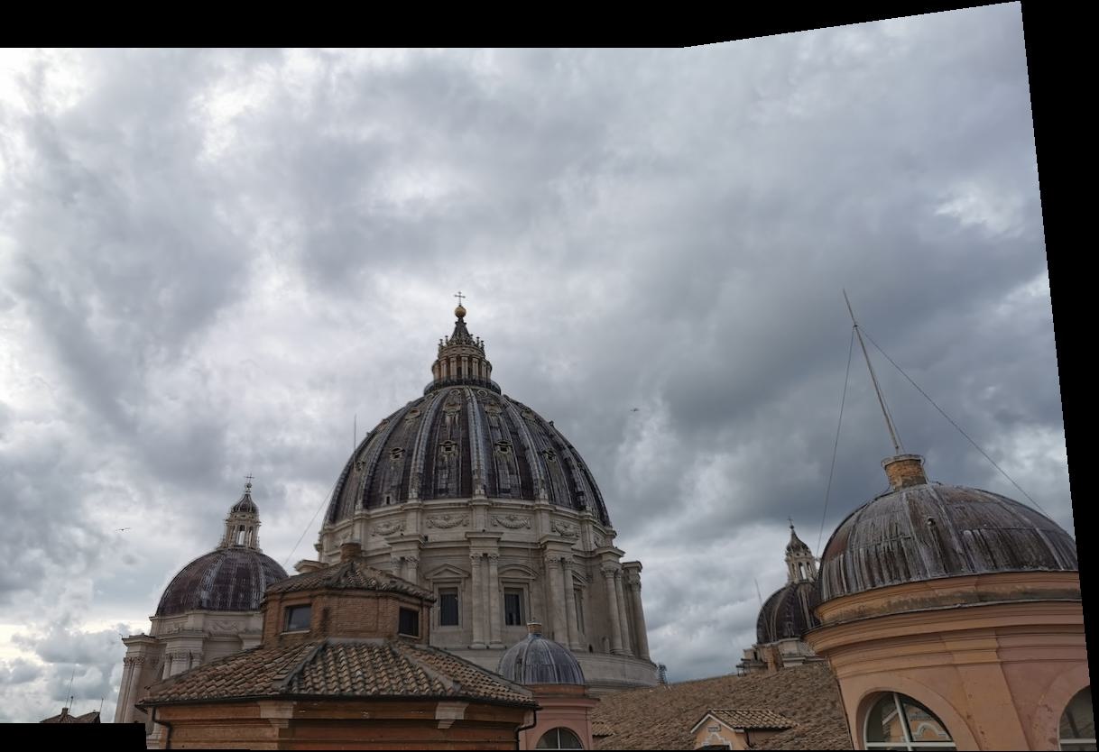
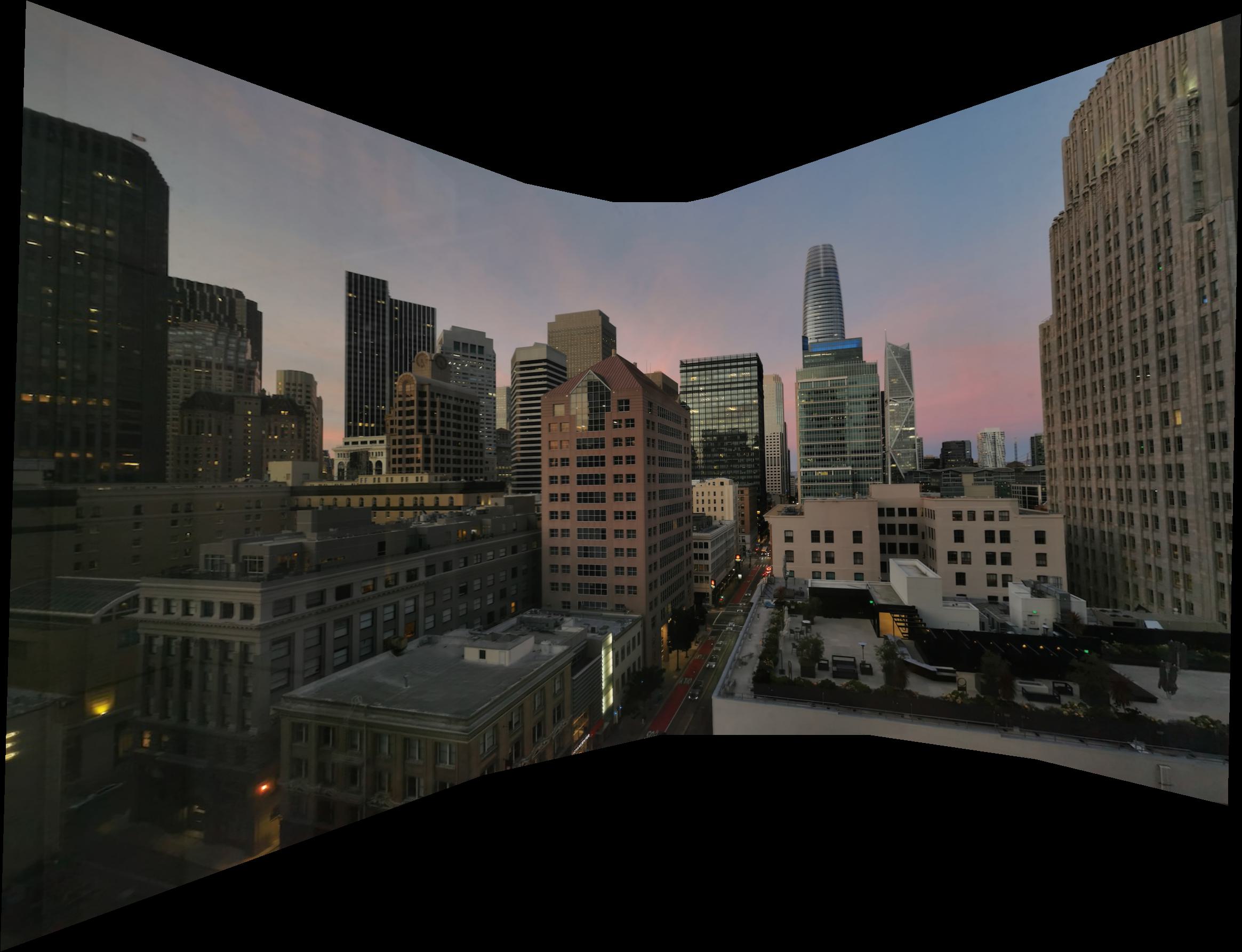
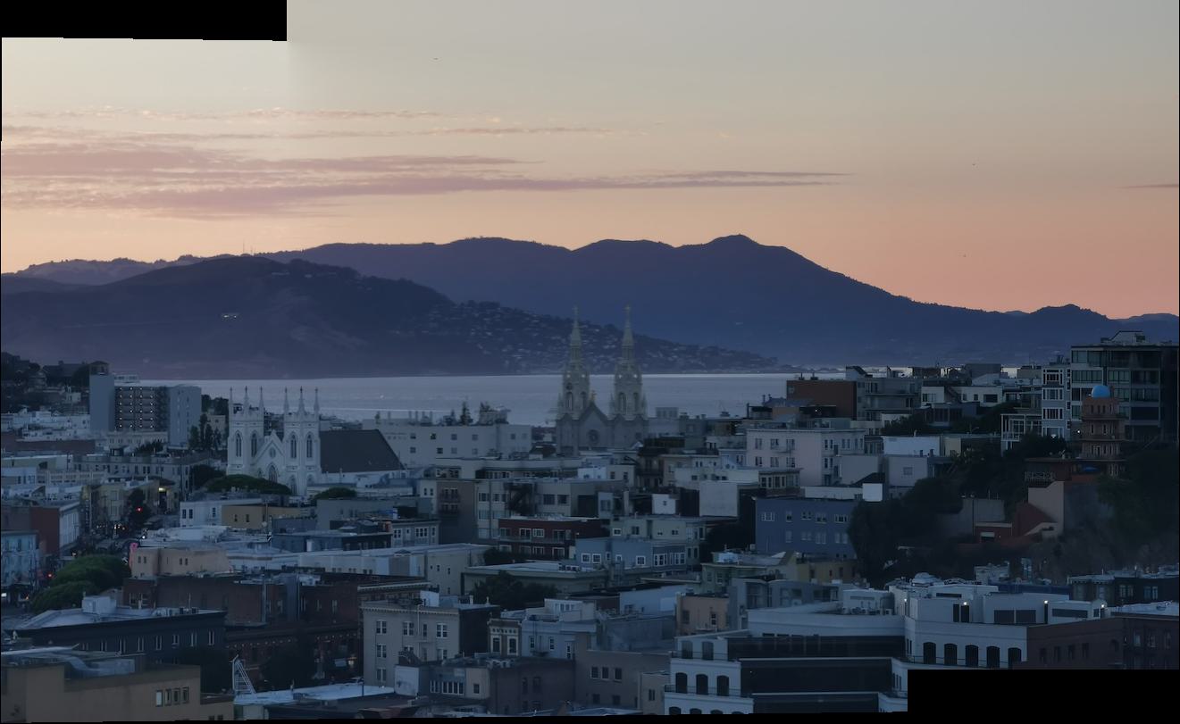
We take several sets of photographs where, within each set, the images are approximately related to each other by camera rotation. Some examples are a sunset view of San Francisco (Fig. 1a), the interior of the Palace Hotel in San Francisco (Fig. 1b), and St. Peter's Basilica in the Vatican City (Fig. 1c).

Legend	Images
Fig. 1a. sf.
Fig. 1b. palace.
Fig. 1c. vatican.

Part 2: Recover Homographies

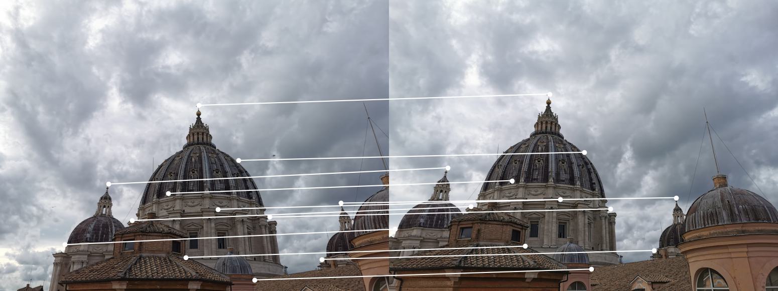
Given a pair of images assumed to be related by a homography, we can estimate the transformation by finding corresponding points (e.g., using a labeling tool developed by a previous student; Fig. 2). In particular, let the homography be parameterized by the matrix \(H=\begin{pmatrix}h_0&h_1&h_2\\h_3&h_4&h_5\\h_6&h_7&1\end{pmatrix}\) that acts on homogeneous coordinates. Given a pair of points \(p_1=\begin{pmatrix}x_1\\y_1\\1\end{pmatrix}\), \(p_2=\begin{pmatrix}x_2\\y_2\\1\end{pmatrix}\) in the two images, a perfect homography transformation should satisfy the equations \(H p_1 = wp_2\), where \(w\) is a scalar. Expanding the matrix multiplication and simplifying, we can rewrite the constraints as \[ \begin{pmatrix} x_1 & y_1 & 1 & 0 & 0 & 0 & -x_1 x_2 & -y_1 x_2\\ 0 & 0 & 0 & x_1 & y_1 & 1 & -x_1 y_2 & -y_1 y_2 \end{pmatrix} \begin{pmatrix} h_0\\h_1\\h_2\\h_3\\h_4\\h_5\\h_6\\h_7 \end{pmatrix} = \begin{pmatrix} x_2\\y_2 \end{pmatrix} \] In general, we can define more than four pairs of corresponding points, obtain an overconstrained system of equations (namely, a stack of pairs of equations of the above form), and solve for an approximate homography using least squares.

Fig. 2. Example corresponding points.

Part 3: Warp the images

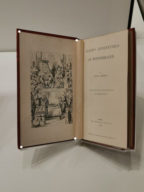
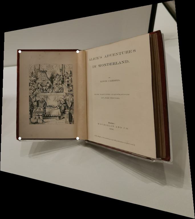
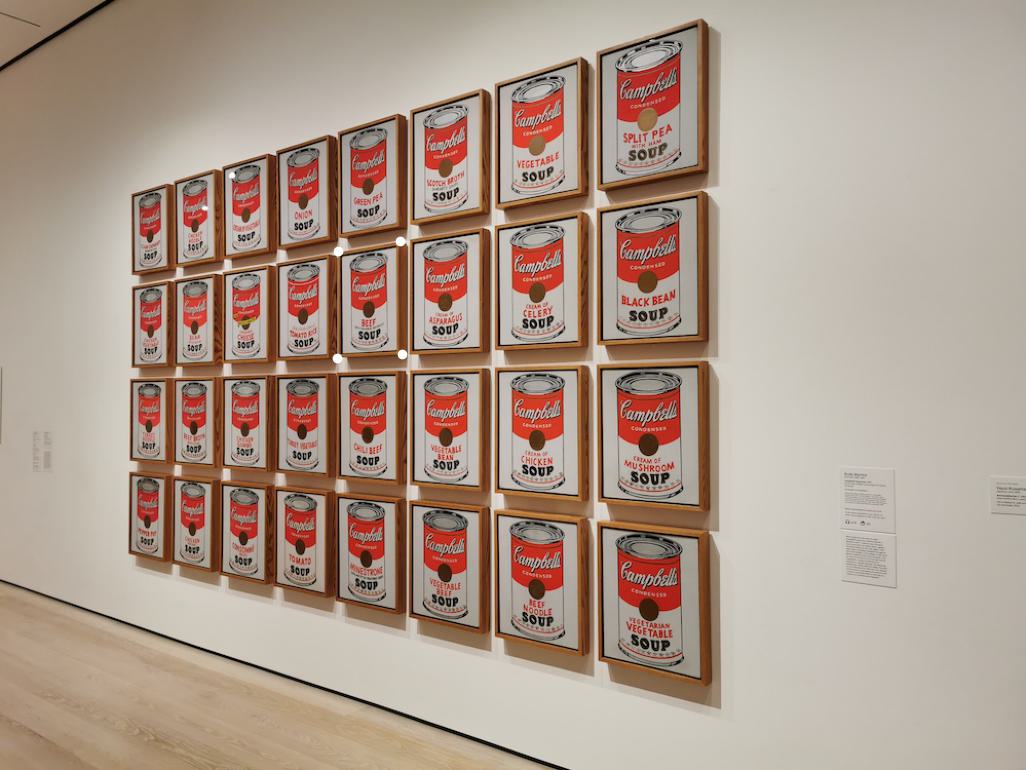
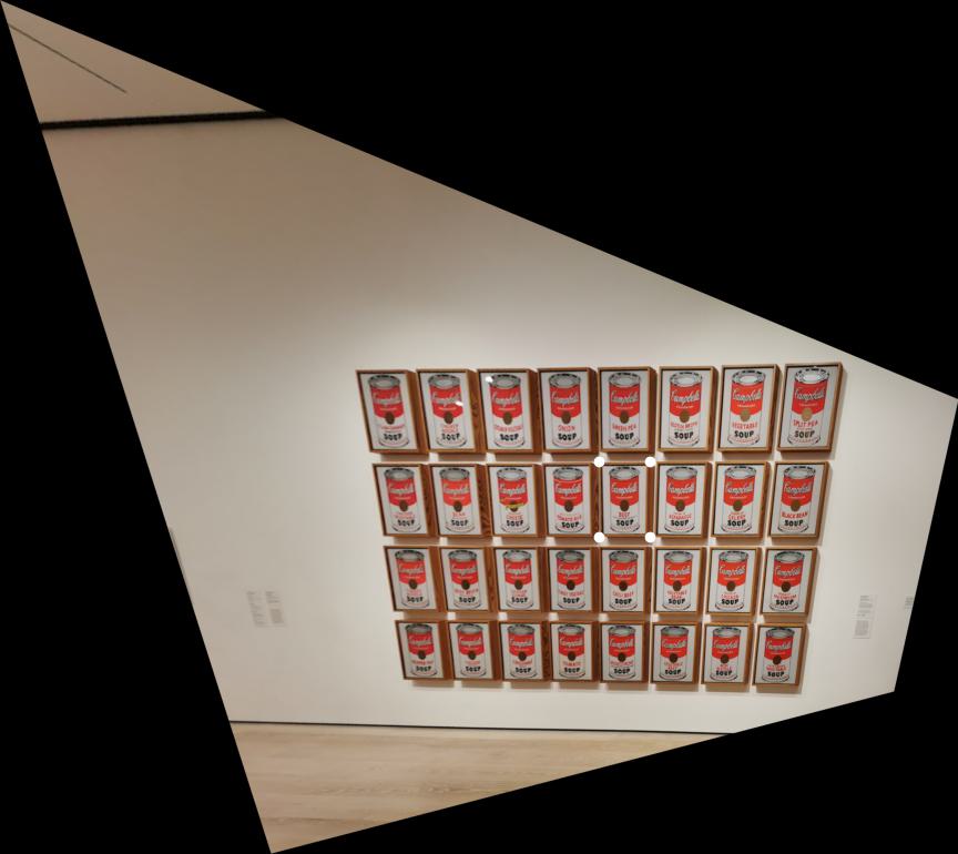
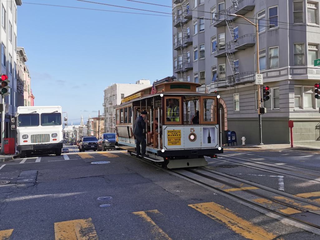
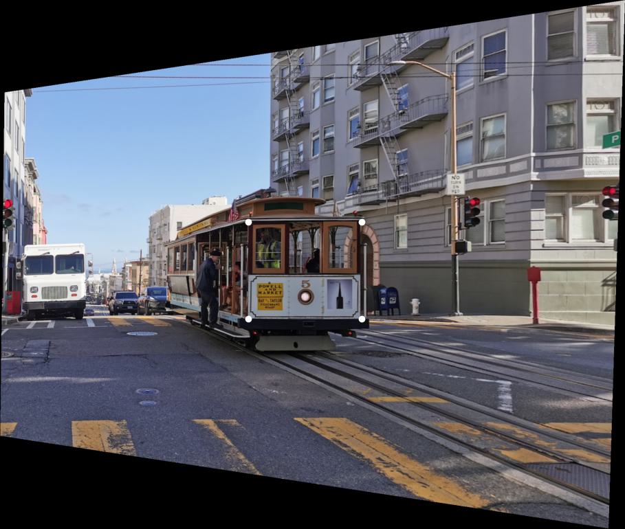
Given a homography, we can transform one image to another camera projection through inverse warping. In particular, we can rectify an image by warping a quadrilateral to a rectangle (Fig. 3a-c).

Legend	Original	Rectified
Fig. 3a. alice.
Fig. 3b. campbell.
Fig. 3c. cablecar.

Part 4: Blend images into a mosaic

To create a mosaic, we transform each image in the set to a common projection (e.g., one of the images). For far apart images that do not have direct corresponding points, we can compute the composition of several homographies using intermediate images. We use a weighted average of the pixel values of images that overlap at a given location (after transforming each individual image). 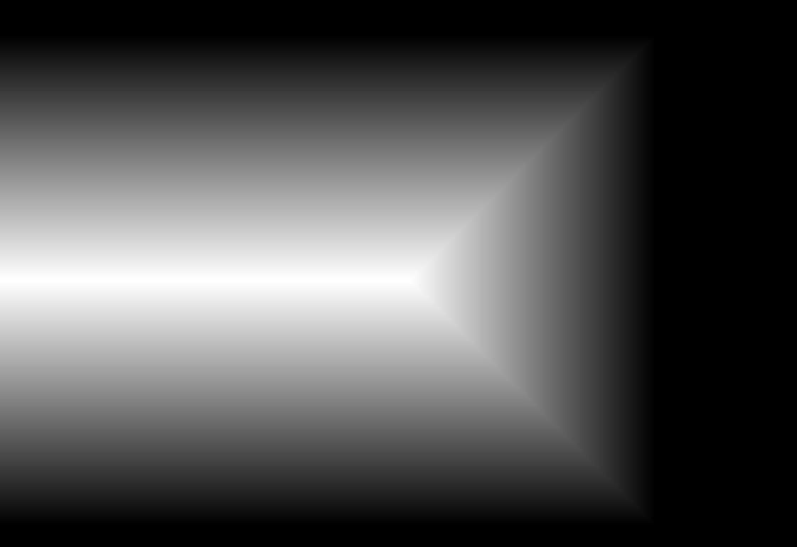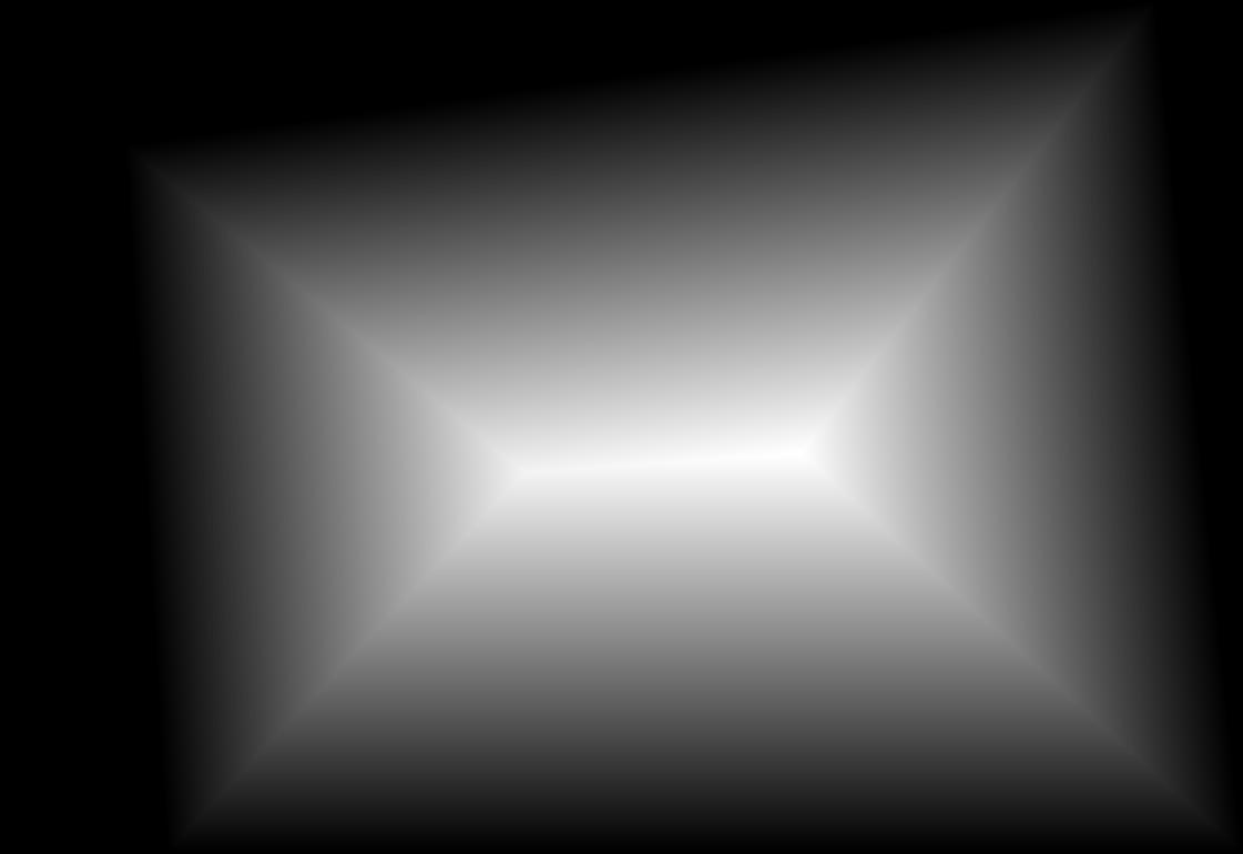In particular, for each pixel \(x=(i,j)\), let \[\alpha_{x}^{(n)}=\frac{d_{x}^{(n)}}{\sum_{n}d_{x}^{(n)}}\] Where \(\alpha_{x}^{(n)}\) is the weight of the \(n\)th image for this pixel, and \[d_{x}^{(n)}=\begin{cases}\inf_{p\in \partial (H_nI_n)}\|p-x\|_2,\ x\in H_nI_n\\ 0,\ x\not\in H_nI_n\end{cases}\] Is the Euclidean distance of the pixel to the boundary \(\partial(\cdot)\) of the transformed image \(I_n\) under homography \(H_n\). Example distance transforms are shown in Fig. 4.

Fig. 4a. \(d\) for vatican_1.	Fig. 4a. \(d\) for vatican_2.

We can then take the weighted average of the pixel values of the images at each pixel location to create the final mosaic (Fig. 5a-c).

Fig. 5a. sf composite.	Fig. 5b. palace composite.	Fig. 5c. vatican composite.

Project 4B: Feature matching for autostitching

In the following parts, we follow the logic of Brown et al., CVPR 2005 to automatically detect and match corner features in pairs of images. These feature pairs can be used as corresponding points to compute homographies and generate image mosaics in a scalable manner. We use the below two photos of sunset to demonstate each step (Fig. 6a-b).

Fig. 6a. sunset_1	Fig. 6b. sunset_2

Part 1: Detecting corner features in an image

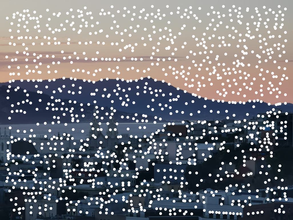
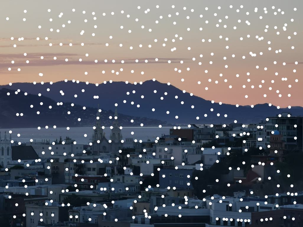
We use the Harris interest point detector (provided implementation) to find corners in an image (Fig. 7a). We used \(\sigma=4\) for the Harris detector to obtain a reasonable density of points in the images. We use adaptive non-maximal suppression to select a subset of the detected corners (Fig. 7b). Specifically, for each corner \(x_i\in\mathcal{H}\) detected by the Harris detector, we compute \[r_i=\min\left\{\{\|x_i-x_j\|_2\mid x_j\in\mathcal{H}, H[x_i] < cH[x_j]\}\cup\{\infty\}\right\}\] as the minimum suppression radius for point \(x_i\), where \(H\) is the Harris matrix, \(\mathcal{H}\) is the set of Harris corners, and \(c\) is a robustness coefficient (we use \(c=0.9\)). We then output the subset of \(N=500\) corners with the largest suppression radii.

Fig. 7a. Harris of sunset_1.	Fig. 7b. ANMS of sunset_1.

Part 2: Extracting a feature descriptor for each feature point

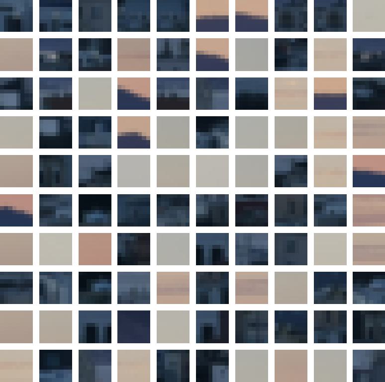
We extract axis-aligned \(40\times 40\)-pixel patches around each feature point, and downsample (with anti-aliasing) to \(8\times 8\) pixels. \(100\) example patches for sunset_1 are shown in Fig. 8.

Fig. 8. Example patches for sunset_1.

Part 3: Matching these feature descriptors between two images

To find potential corresponding points between two images, we compute the pairwise Euclidean distance between the feature descriptors of the two images. To reduce outliers, we use Lowe's technique as in the paper: for each point in the first image, we find the two nearest neighbors (NN) in the set of feature points in the second image. 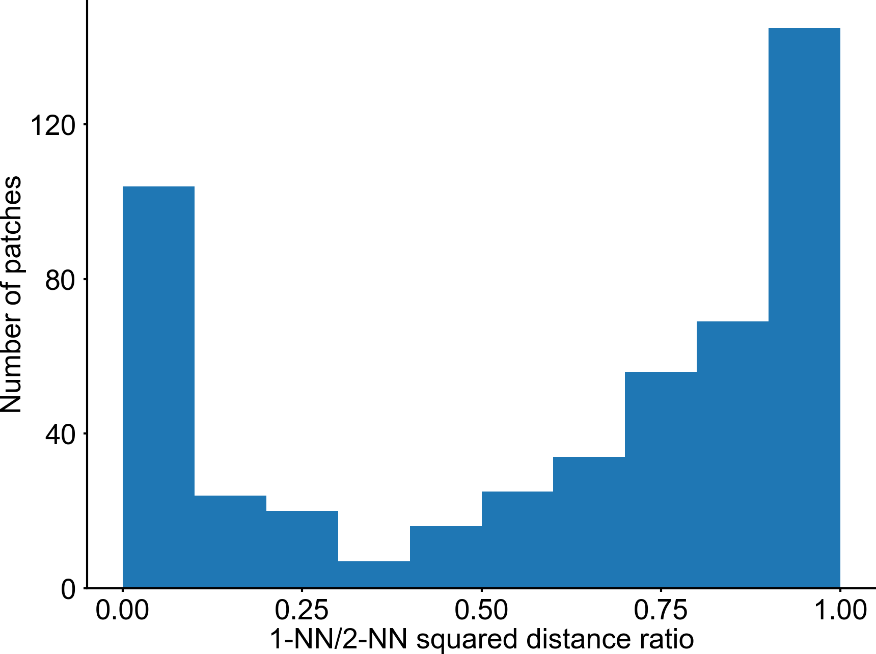We then compute the ratio of the squared Euclidean distance to the first and second NNs, and only store this match if the ratio is less than a threshold (we use \(0.2\), which was empirically found to be a reasonable threshold both in Fig. 6 in the paper and by inspecting a distribution of ratios on our images; see Fig. 9a). 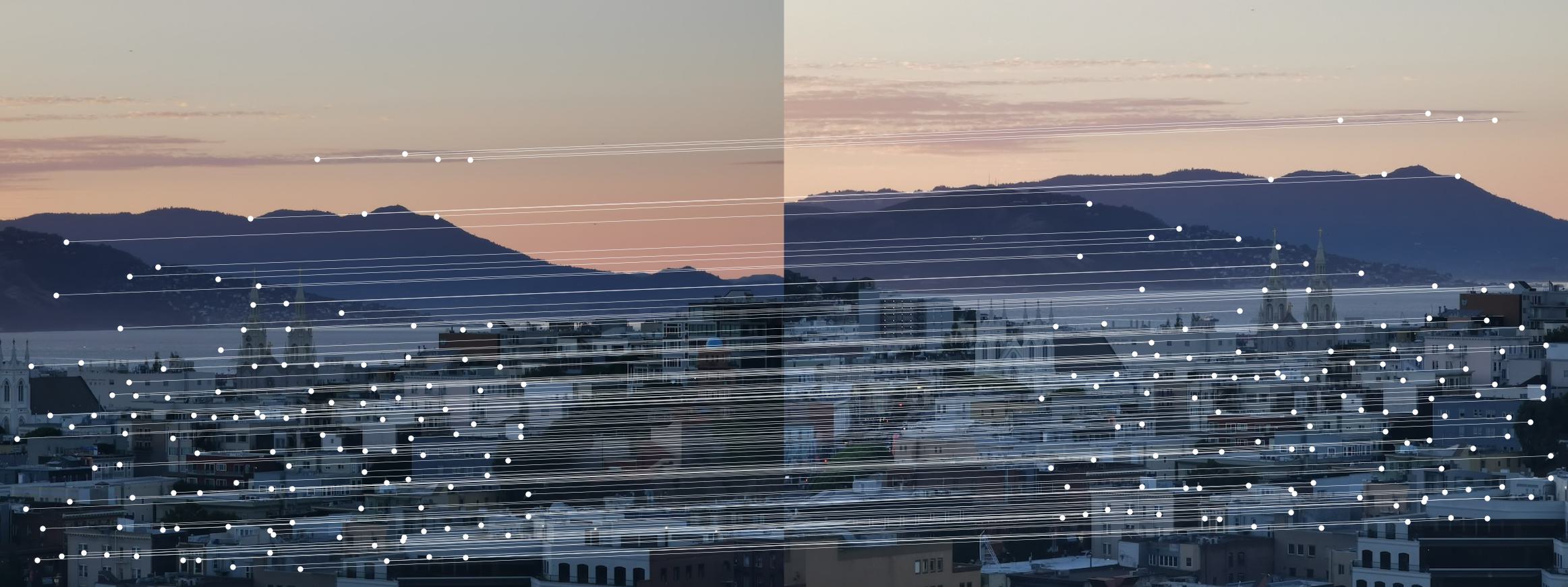Final matches obtained are shown in Fig. 9b.

Fig. 9a. 1-NN and 2-NN squared distance ratios for sunset.	Fig. 9b. Matching points for sunset.

Part 4: Use a robust method (RANSAC) to compute a homography

To compute a robust homography from the automatically detected feature matches, we use a \(4\)-point RANSAC algorithm. Specifically, we randomly sample \(4\) pairs of feature points, compute the homography from these pairs, apply this homography to all matched points, and count the number of inliers (points where the actual match is less than \(d\) pixels away from the transformed match using this homography). We repeat this process for \(N\) iterations, and output the maximal set of inliers. This set is then used to compute the final homography through least squares. We use \(N=1000\) and \(d=3\) below, and obtain the corresponding points as in Fig. 10 (note that Lowe's technique already gives a reasonable set of corresponding points, so the additional filtering from RANSAC appears minimal here).

Fig. 10. Final matching points for sunset.

Part 5: Proceed as in the first part to produce a mosaic

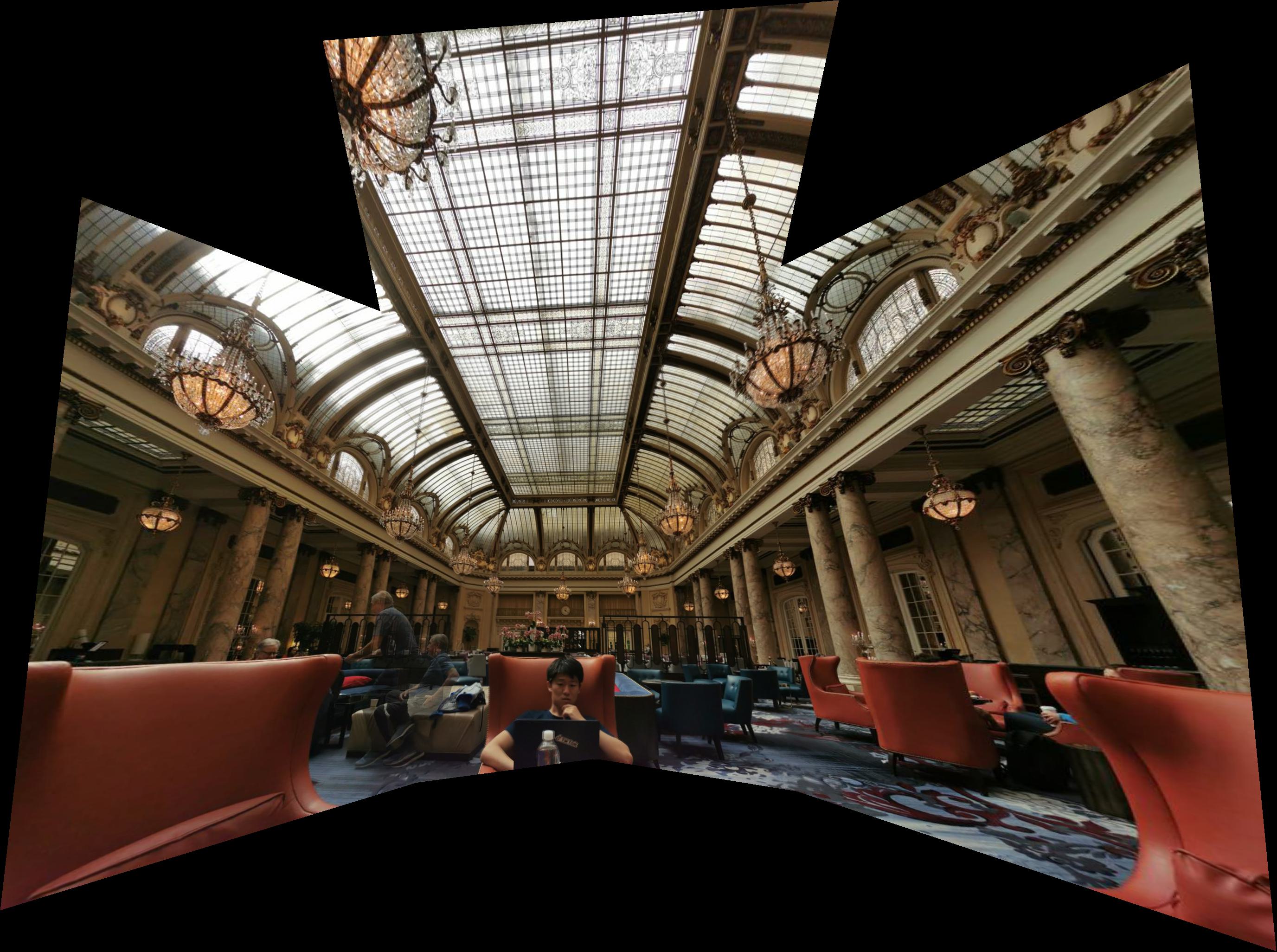
Using the homography computed from the automatically detected feature matches, we can proceed as in the first part to produce a mosaic (Fig. 11a-c).

Legend	Manual	Automatic
Fig. 11a. sf.
Fig. 11b. palace.
Fig. 11c. vatican.

Automation enables scalability, so more examples of visually appealling image mosaics are shown below (Fig. 12 a-e).

Legend	Automatic Mosaic
Fig. 12a. Full sf.
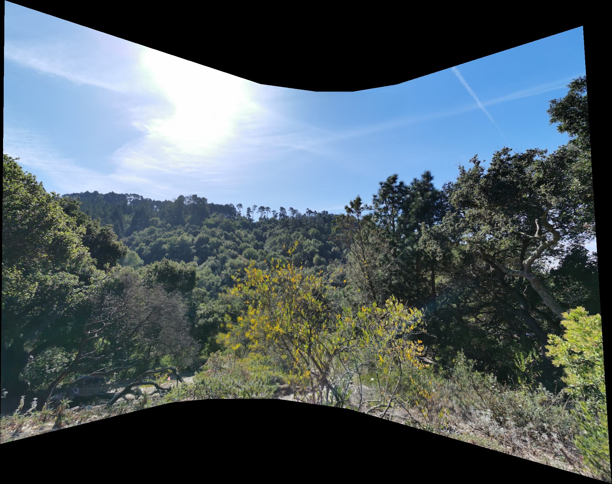
Fig. 12b. botanical-garden.
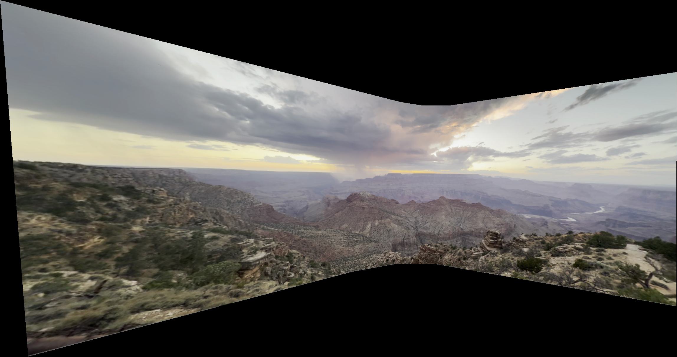
Fig. 12c. canyon. (Photos by R. Sun)
Fig. 12d. sunset.

Comment: Combining shadows of a whole

Photography is inherently a lossy projection of the world, since it captures a single perspective, with limited field of view, of the entire world. Reconstructing the world (e.g., parameterized by the plenoptic function) is therefore an ill-posed inverse problem, as individual photographs have much lower expressivity than the world. Indeed, our photograph mosaic is an attempt to increase the expressivity of photography by combining multiple views through homography transforms (which are good models of image reprojection caused by camera rotation). Moreover, feature matching that enables homography estimation crucially relies on the assumption that the underlying world is static, and that the features are sufficiently sparsely distributed so that a nearest-neighbor search can comfortably return the correct corresponding points.
Philosophically, it is tempting to draw an analogy with Plato, where the world is an ideal form and photography a process of obtaining shadows (imperfect instantiations or projections) of this form, not unlike those in the Allegory of the Cave. Image mosaicing, then, is perhaps an ultimately futile (since the world is so much richer than any combination of 2D photographs), but nonetheless noble, attempt of rising above shadows to approximate the true form.